Paths and Trajectories

Klamp’t distinguishes between paths and trajectories: paths are geometric, time-free curves, while trajectories are paths with an explicit time parameterization. Mathematically, paths are expressed as a continuous curve

\(y(s):[0,1] \rightarrow C\)

while trajectories are expressed as continuous curves

\(y(t):[t_i,t_f] \rightarrow C\)

where \(C\) is the configuration space and \(t_i,t_f\) are the initial and final times of the trajectory, respectively.

Classical motion planners compute paths, because time is essentially irrelevant for fully actuated robots in static environments. However, a robot must ultimately execute trajectories, so a planner must somehow prescribe times to paths before executing them. Various methods are available in Klamp’t to convert paths into trajectories.

Path and trajectory representations

Type	Continuity	Timed?	Description
Configs	C0	No	The simplest path type: a list of Config milestones* that should be piecewise linearly interpolated. These are outputted from kinematic motion planners.
Piecewise linear	C0	Yes	Given by lists of times and milestones that should be piecewise linearly interpolated. The most compatible trajectory type. Implemented for Euclidean spaces via the :class:~`klampt.model.trajectory.Trajectory` class
Cubic spline	C1	Yes	Piecewise cubic curve, with time. Implemented for Euclidean spaces by :class:~`klampt.model.trajectory.HermiteTrajectory`.
MultiPath	C0 or C1	Either	A rich container type for paths/trajectories annotated with changing contacts and IK constraints.

Note

To properly handle a robot’s rotational joints, milestones should be interpolated via robot-specific interpolation functions. Cartesian linear interpolation does not correctly handle floating and spin joints. We provide the RobotTrajectory class to do this automatically.

For legged robots and multi-step manipulations, the preferred path type is MultiPath, which allows storing both untimed paths and timed trajectories. It can also store multiple path sections with inverse kinematics constraints on each section. More details on the MultiPath type are given below.

API summary

The code for implementing klampt.model.trajectory. Piecewise linear trajectories are given in the Trajectory class. Paths in non-Euclidean spaces are represented by the SO3Trajectory, SE3Trajectory, and RobotTrajectory classes.

Members include:

• times: an array of N floats, in increasing order, listing points in time.

• milestones a list of N Config milestones reached at each of those times.

Typically, a trajectory has times[0]=0, but this is not required.

The difference between these classes is the space in which “straight line” interpolation is performed.

• The standard Trajectory class assumes the space is an N-D Euclidean space.

• RobotTrajectory requires that each milestone is a Config for the specified robot. It will also take any special joints, like freely-rotating joints, into account during interpolation, so that, for example, a mobile base robot will interpolate its orientation DOF from 0.1 radians to 6.1 radians the “short way around”.

• SO3Trajectory interpolates in SO(3), in the space of rotation matrices. Each milestone is a 9-element rotation matrix (see the so3 module) and interpolation is performed using geodesics in SO(3).

• SE3Trajectory interpolates in SE(3), in the space of rigid transforms. Each milestone is a 12-element rotation matrix + translation vector concatenated together (see the se3 module) and interpolation is performed using geodesics in SE(3).

The basic API uses the following methods:

• traj = Trajectory(): constructs an empty trajectory. You will need to populate the times and milestones attributes before using any other methods.

• traj = Trajectory([t0,t1,...,tn],[q0,q1,...qn]): constructs a trajectory with times t0,t1,…tn and milestones q0,q1,…qn.

• traj = Trajectory(milestones=[q0,q1,,...,qn]): constructs a trajectory with milestones q0,q1,…,tn and default uniform timing, times 0,1,…,n.

• traj.eval(t): evaluates the trajectory, handling out-of-bounds times by clamping. O(log n) time, where n is the number of milestones.

• traj.eval(t,'loop'): evaluates the trajectory, handling out-of-bounds times by cycling.

• traj.deriv(t): evaluates the trajectory derivative, handling out-of-bounds times by clamping. O(log n) time, where n is the number of milestones.

• traj.deriv(t,'loop'): evaluates the trajectory derivative, handling out-of-bounds times by cycling.

• traj.start/endTime(): returns the start/end time.

• traj.duration(): returns traj.endTime()-traj.startTime().

• traj.load/save(fn): loads / saves to a file on disk.

Trajectories can also be modified through concatenation and splicing operations:

• traj.concat(suffix,relative=False,jumpPolicy='strict'): appends a suffix Trajectory onto this one.

• traj.before/after(t): returns the portion of the path before and after time t.

• traj.split(t): equivalent to (traj.before(t),traj.after(t))

• traj.splice(suffix,time=None,relative=False,jumpPolicy='strict'): splices another Trajectory onto this one at a given time.

The relative parameter, if set to True, means that the suffix starts at time 0, but should be time-shifted so that it starts at the given insertion time. jumpPolicy='strict' means that an exception will be thrown if the suffix does not match the trajectory at the insertion time

The knot points in the time domain can also be revised without modifying the shape of the path (much):

• traj.insert(t): inserts a milestone at time t, if one doesn’t exist.

• traj.discretize(dt): makes milestones evenly spaced in time, with time dt apart. This might slightly change the shape of the path.

• traj.remesh(times): inserts new milestones at each of the points in times. Equivalent to for t in times: traj.insert(t), but faster.

Hermite spline interpolation is available in the HermiteTrajectory class in klampt.model.trajectory. You may either set tangents manually or automatically using the makeSpline method, as follows:

from klampt.model import trajectory

traj = trajectory.Trajectory()
#... set up traj
traj2 = trajectory.HermiteTrajectory()
traj2.makeSpline(traj)

For non-Euclidean Hermite splines, you may use the GeodesicHermiteTrajectory representation. The SO3HermiteTrajectory and SE3HermiteTrajectory classes are available for smooth curves in SO(3) and SE(3). [New in 0.8.3]

Conversions

Conversions between path types are found in klampt.model.trajectory.

In particular the path_to_trajectory() method converts an untimed path into a timed trajectory. This has many options, and the example program path_test.py demos several of these options.

To convert from a cubic trajectory to an approximate linear trajectory, the discretize_config method should be used.

To get the SE(3) trajectory of a link’s transform as the robot follows a RobotTrajectory, use RobotTrajectory.getLinkTrajectory(link,dt). Here, dt is a discretization resolution. To further convert this to the trajectory of the position of a point on the link, use RobotTrajectory.getLinkTrajectory(link,dt).getPositionTrajectory(localPt), where localPt gives the local coordinates of the point.

Example

It is a common task to take a sequence of waypoints, either from a planner or from manual editing, and convert them into a timed trajectory to be executed.

A list of waypoints is also known as a Configs object. We will first define 7 milestones manually, on an XZ plane:

from klampt.model import trajectory

milestones = [[0,0,0],[0.02,0,0],[1,0,0],[2,0,1],[2.2,0,1.5],[3,0,1],[4,0,-0.3]]

Now let’s create a Trajectory out of it. The constructor will just assign a default timing, which is uniformly spaced in time.

traj = trajectory.Trajectory(milestones=milestones)

Now, let’s see how the eval function works:

#prints milestones 0-5
print(0,":",traj.eval(0))
print(1,":",traj.eval(1))
print(2,":",traj.eval(2))
print(3,":",traj.eval(3))
print(4,":",traj.eval(4))
print(5,":",traj.eval(5))
print(6,":",traj.eval(6))
#print some interpolated points
print(0.5,":",traj.eval(0.5))
print(2.5,":",traj.eval(2.5))
#print some stuff after the end of trajectory
print(7,":",traj.eval(7))
print(100.3,":",traj.eval(100.3))
print(-2,":",traj.eval(-2))

OK, that seems reasonable. But it’s a little hard to understand what this looks like through text printouts. Let’s use the visualization to see how this path behaves:

from klampt import vis

vis.add("point",[0,0,0])
vis.animate("point",traj)
vis.add("traj",traj)
vis.spin(float('inf'))   #show the window until you close it

This will pop up a visualization, show the path, and animate a point along it as well.

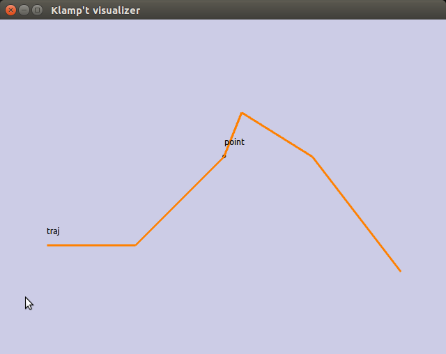
It looks a little like a mountain, and the point moves slowly at the start before moving along the curve.

Let’s now look at what happens when we convert this to a HermiteTrajectory…

traj2 = trajectory.HermiteTrajectory()
traj2.makeSpline(traj)

vis.animate("point",traj2)
vis.add("traj2",traj2)
vis.spin(float('inf'))

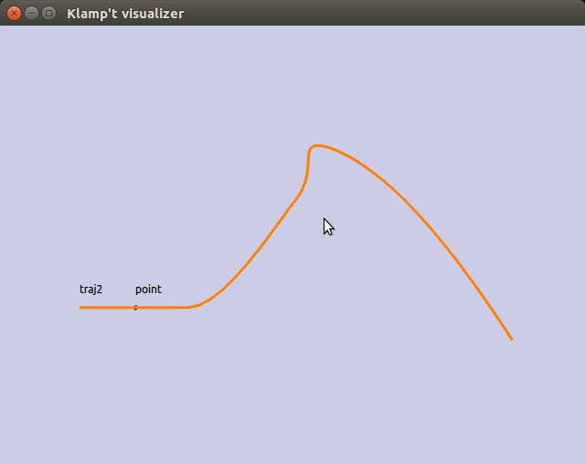
Now the point curves smoothly through the milestones we defined!

Finally we might want to address the problem that the milestones are executed uniformly in the time domain, even though the first two milestones are identical. The path_to_trajectory() function has a whole host of options, and you can play around with them until you get the results that you want.

traj_timed = trajectory.path_to_trajectory(traj,vmax=2,amax=4)
#next, try this line instead
#traj_timed = trajectory.path_to_trajectory(traj,timing='sqrt-L2',speed='limited',vmax=2,amax=4)
#or this line
#traj_timed = trajectory.path_to_trajectory(traj2.discretize(0.1),timing='sqrt-L2',speed=0.3)
vis.animate("point",traj_timed)
vis.spin(float('inf'))

Visual keyframe editing

Trajectories can be edited as keyframes in klampt_browser or Python code.

As an example of using klampt_browser, run the following script in a command-line terminal:

cd Klampt-examples/data
klampt_browser athlete_plane.xml

Then expand the “motions” directory and click on one of the motions, such as athlete_flex.path. Then, click the Edit button. You may modify milestones and timing by hand, and save the edited path back to disk.

In Python code, the same effect is achieved by the klampt.io.resource.edit() function.

from klampt.io import resource

save,result = resource.edit("my trajectory",traj,world=world)
if save:
    #the user pressed 'OK'
    traj = result
    #do something with the result, e.g., save it to disk
    from klampt.io import loader
    loader.save(traj,'Trajectory','mytraj.path')
else:
    #the user pressed 'Cancel'.  result is the last state of the edited trajectory
    pass

Multipaths

A MultiPath is a rich path representation for legged robot motion. They contain one or more path(or trajectory) sections along with a set of IK constraints and holds that should be satisfied during each of the sections. This information can be used to interpolate between milestones more intelligently, or for controllers to compute feedforward torques more intelligently than a raw path. They are loaded and saved to XML files.

Each MultiPath section maintains a list of IK constraints in the ikObjectives member, and a list of Holds in the holds member. There is also support for storing common holds in the MultiPaths holdSet member, and referencing them through a section’s holdNames or holdIndices lists (keyed via string or integer index, respectively). This functionality helps determine which constraints are shared between sections, and also saves a bit of storage space.

MultiPaths also contain arbitrary application-specific settings, which are stored in a string-keyed dictionary member settings. Common settings include:

• robot, which indicates the name of the robot for which the path was generated.

• resolution, which indicates the resolution to which a path has been discretized. If resolution has not been set or is too large for the given application, a program should use IK to interpolate the path.

• program, the name of the procedure used to generate the path.

• command_line, the shell command used to invoke the program that generated the path.

Sections may also have custom settings. No common settings have yet been defined for sections, these are all application-dependent.

API summary

Details can be found in the MultiPath documentation.

The klampt_path script can also be run to perform various simple transformations and conversions on MultiPaths.

Also, you may see the utility scripts in

Klampt-examples/Python3/utils/multipath\_to\_timed\_path.py

for an example of assigning times to a multipath.

Cartesian Trajectories

A number of Cartesian path generation functions are available in the cartesian_trajectory module.

See the Control manual for more detail about Cartesian motion execution.

Trajectory Execution

Sending to a Klamp’t simulated robot

The simplest way to send a path to a SimRobotController is to use execute_path() (untimed path). You can also use path_to_trajectory() to generate a timed trajectory, then execute_trajectory().

For greater control, you may either run an eval(t) loop to send position commands, or use the controller motion queuing process.

If you have built or installed the Klampt binaries, you may use the SimTest program to observe a trajectory in simulation. Save the trajectory to disk as a Trajectory file and the starting Config as follows:

from klampt.io import loader
loader.save(traj,'Trajectory','my_traj.path')
loader.save(traj.milestones[0],'Config','my_traj_start.config')

then run

SimTest [world file] -path [name of path file] -config [start config]

Sending to a real robot

To send a Trajectory to your own robot, you can either 1) build your own control loop or 2) build a Robot Interface Layer object.

If your robot accepts PID commands

Set up a while loop to advance time forward and manually send PID commands, like this:

import time

#this code assumes traj is already given, and your controller provides a function pid_command(q,dq)

def convert_klampt_config(q):
    """Converts klampt config to my robot's config, e.g., extract DOFs,
    convert units, account for joint offsets.

    Right now, does a straight pass-through.
    """
    return q

def convert_klampt_velocity(dq):
    """Converts klampt velocity to my robot's velocity, e.g., extract DOFs,
    convert units.

    Right now, does a straight pass-through.
    """
    return dq

dt = 0.01  #approximately a 100Hz control loop
t0 = time.time())
while True:
    t = time.time()-t0
    if t > traj.endTime():
        break
    qklampt = traj.eval(t)
    dqklampt = traj.eval(t)
    qrobot = convert_klampt_config(qklampt)
    dqrobot = convert_klampt_velocity(dqklampt)
    pid_command(qrobot,dqrobot)
    time.sleep(dt)
print("Done")

If your robot accepts queued, timed waypoints

Feed each of the trajectory milestones to the robot’s queue, like this:

#this code assumes traj is already given, and your controller provides a function queue_move(q,duration)
move_home_duration = 10  #moves slowly to the home configuration over 10 seconds
lastt = None
for t,q in zip(traj.times,traj.milestones):
    if lastt is None:
        queue_move(q,move_home_duration)
    else:
        queue_move(q,t-lastt)
    lastt = t

If your robot uses ROS JointTrajectory messages

Set up a ROS publisher, and run the conversion utilities in klampt.io.ros:

import rospy
from klampt import io

ros_publisher = rospy.Publisher(TOPIC,...args...)
link_joint_names = [... the list of ROS joints corresponding to Klamp't DOFs...]
msg = io.ros.to_JointTrajectory(traj,link_joint_names=link_joint_names)
ros_publisher.publish(msg)

If you have a Robot Interface Layer class

Use the setPiecewiseLinear() function, as follows:

ril = MyRobotInterfaceLayer()
if not ril.initialize():
    raise RuntimeError("Couldn't initialize my robot")
ril.setPiecewiseLinear(traj.times,traj.milestones)