Math concepts
Klamp’t assumes basic familiarity with 3D geometry and linear algebra concepts. It heavily uses structures that representing vectors, matrices, 3D points, 3D rotations, and 3D transformations. These routines are heavily tested and fast.
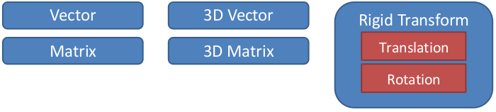
The main mathematical objects used in Klampt are as follows:
Vector: a variable-length (n-D) vector.Matrix: a variable-size (m x n) matrix.Vector3: a 3-D vector.Matrix3: a 3x3 matrix.Rotation: a 3D rotation, specifically an element of the special orthogonal group SO(3), usually represented by aMatrix3.RigidTransform: a rigid transformationT(x) = R*x + t, withRa rotation andtaVector3
API summary
3D math operations are found in the klampt.math module under the following files.
vectorops: basic vector operations on lists of numbers.
so2: routines for handling 2D rotations.
so3: routines for handling 3D rotations.
se3: routines for handling 3D rigid transformations
The use of numpy / scipy is recommended if you are doing any significant linear algebra. We provide converters from Klampt math objects to numpy objects.
3D Points / Directions
The Klamp’t Python API represents points and directions simply as 3-lists or 3-tuples of floats. To perform operations on such objects, the klampt.math.vectorops module has functions for adding, subtracting, multiplying, normalizing, and interpolating. To summarize, the following table lists major vector operations in Matlab, the Klamp’t vectorops module, and Numpy/Scipy.
Operation |
Matlab |
Klamp’t vectorops |
Numpy/Scipy |
|---|---|---|---|
Import |
N/A |
from klampt.math import vectorops |
import numpy |
Create vector from list of elements |
a=[1 2 3]; |
a=[1,2,3] |
a=numpy.array([1,2,3]) |
Copy vector |
b=a; |
b=a[:] |
b=a.copy() or b=numpy.array(a) |
Create vector of zeros |
a=zeros(3,1); |
a=[0]*3 |
a=numpy.zeros(3) or a=numpy.array([0]*3) |
Access first element |
a(1) |
a[0] |
a[0] |
Concatenate two vectors |
[a b] |
a+b |
concatenate((a,b)) |
Getting elements as a Python list |
N/A |
a |
a.tolist() |
Add vectors |
a+b |
vectorops.add(a,b) |
a+b |
Subtract vectors |
a-b |
vectorops.sub(a,b) |
a-b |
Multiply vector by scalar |
a*b |
vectorops.mul(a,b) |
a*b |
Divide vector by scalar |
a/b |
vectorops.div(a,b) |
a/b |
Add vector to vector times scalar (multiply-add) |
a+b*c |
vectorops.madd(a,b,c) |
a+b*c |
Incremental add vectors |
a=a+b; |
a=vectorops.add(a,b) |
a+=b |
Incremental subtract vectors |
a=a-b; |
a=vectorops.sub(a,b) |
a-=b |
Incremental multiply vector by scalar |
a=a*b; |
a=vectorops.mul(a,b) |
a*=b |
Incremental divide vector by scalar |
a=a/b; |
a=vectorops.div(a,b) |
a/=b |
Elementwise multiply vectors |
a.*b; |
vectorops.mul(a,b) |
a*b or numpy.multiply(a,b) |
Dot product |
dot(a,b); |
vectorops.dot(a,b) |
numpy.dot(a,b) |
L2 norm |
norm(a); |
vectorops.norm(a) |
numpy.linalg.norm(a) |
Squared L2 norm |
norm(a)^2 or dot(a,a) |
vectorops.normSquared(a) (faster than norm) |
numpy.linalg.norm(a)**2 |
L2 distance |
norm(a-b) |
vectorops.distance(a,b) |
numpy.linalg.norm(a-b) |
Squared L2 distance |
norm(a-b)^2 or dot(a-b,a-b) |
vectorops.distanceSquared(a) (faster than distance) |
numpy.linalg.norm(a-b)**2 |
Cross product |
cross(a,b) |
vectorops.cross(a,b) |
numpy.cross(a,b) |
Interpolate between vectors a and b with parameter u |
a+u*(b-a) |
vectorops.interpolate(a,b,u) |
a+u*(b-a) |
Matrix-vector multiply |
A*b |
[vectorops.dot(ai,b) for ai in A] |
numpy.dot(A,b) |
3D Rotations
The Klamp’t Python API represents a 3D rotation as a 9-tuple
(a11,a21,a31,a21,a22,a32,a31,a32,a33) listing each of the entries of the
rotation matrix
\(\begin{bmatrix} a11 & a12 & a13 \\ a21 & a22 & a23 \\ a31 & a32 & a33 \end{bmatrix}\)
in column-major order. The
klampt.math.so3 module provides several operations on rotations
in this representation,
as well as conversions to and from alternate representations. (The so3
module is so named because the space of rotations is known as the
special orthogonal group SO(3)).
For some basic operation, try the following code:
from klampt.math import so3,vectorops

    A = so3.identity()  #builds an identity rotation
    print("Original:",A)  #prints [1,0,0,0,1,0,0,0,1]
    #pretty-print the rotation matrix
    print("Pretty printed:",so3.__str__(A) )
    #returns the 2D array form of A
    print("matrix()",so3.matrix(A) )

    point = [3.0,1.5,-0.4]  #make some point
    #Apply the rotation A to the point.
    print(so3.apply(A,point)  )
    #Since it's an identity, the point does not change
Try it again with a 90 degree rotation about the z axis, by replacing
the assignment to A with A=[0,1,0,-1,0,0,0,0,1]. Observe
that the printed point is now rotated by 90 degrees from the original
point.
We can also produce rotation matrices using the so3.rotation(axis,angle)
function. The axis is a unit vector (given by a 3-tuple) and the angle
is given in radians. So, to construct the 90 degree rotation about Z we
used above, we can avoid fussing about the ordering of elements in the
9-tuple, by simply using the following code:
import math
from klampt.math import so3

#first argument is the axis, second argument is the angle in radians
print(so3.rotation((0,0,1),math.radians(90)))
Klamp’t also supports conversions to three other commonly used rotation representations: axis-angle, rotation vector (aka exponential map), and quaternions.
Axis-angle representations we have seen above, and are simply a pair
(axis,angle). To convert to/from an so3 element, useso3.from_axis_angle()andso3.axis_angle()Rotation vector representations are very similar to axis-angle representations but are more compact. They are a 3-tuple
(mx,my,mz)equivalent to axis*angle. To convert to/from an so3 element useso3.from_rotation_vector()andso3.rotation_vector().Quaternion representations are 4-tuples
(w,x,y,z)representing a unit quaternion. To convert to/from an so3 element useso3.from_quaternion()andso3.quaternion(). (Note that in some other packages, such as ROS and Scipy, the (x,y,z,w) ordering is used.)
Rotations can also be composed using the so3.mul(A,B) function. Note
that the result corresponds to a rotation first by B, and then by A.
(Recall that rotation composition is not symmetric! so3.mul(A,B) != so3.mul(B,A)
unless the two rotations share the same axis of rotation)
Inversion of a rotation is accomplished via the so3.inv(A) function.
Inversion is equivalent to the matrix transpose, since rotation matrices
are orthogonal.
The space of rotations is fundamentally different from Cartesian space, and hence computing interpolations and finding the difference between rotations is not as simple as taking standard linear interpolations in the 9-D space. The klampt.so3 module provides functionality for properly computing geodesics on SO(3).
from klampt.math import vectorops,so3
import math

A = so3.rotation((0,0,1),math.radians(90))
B = so3.rotation((1,0,0),math.radians(-90))

#WRONG WAY! SO3 is not a cartesian space
#print("Distance:",vectorops.distance(A,B))
#print("Halfway:",vectorops.interpolate(A,B,0.5))
#print("Difference:",vectorops.sub(B,A))

#RIGHT WAY!
print("Distance:",so3.distance(A,B))
print("Start of interpolation:",so3.interpolate(A,B,0))
print("Halfway:",so3.interpolate(A,B,0.5))
print("End of interpolation:",so3.interpolate(A,B,1))
print("Lie derivative:",so3.error(A,B))
The last term is a 3-tuple indicating the amounts by which A would need to be rotated about its local x, y and z axes to get to B.
The following table summarizes the major SO(3) operations in Matlab, the Klamp’t so3 module, Numpy, and Scipy.
Operation |
Matlab (Robotics toolbox) |
Klamp’t so3 |
Numpy |
Scipy |
|---|---|---|---|---|
Import |
N/A |
from klampt.math import so3 |
import numpy |
from scipy.spatial.transform import Rotation as R |
Create SO(3) identity |
eye(3) |
so3.identity() |
numpy.eye(3) |
R.from_rotvec([0,0,0]) |
Create SO(3) from 3x3 matrix |
a |
so3.from_matrix(a) |
a |
a.from_dcm() |
Create from axis-angle representation |
axang2rotm([x y z rads]) |
so3.rotation([x,y,z],rads) |
N/A |
R.from_rotvec([x*r,y*r,z*r]) |
Create from rotation vector representation |
rads=norm(w); axang2rotm([w/rads rads]) |
so3.from_rotation_vector(w) |
N/A |
R.from_rotvec(w) |
Create from euler-angle representation |
eul2rotm([theta phi psi],’ZYX’) |
so3.from_rpy((psi,phi,theta)) |
N/A |
R.from_euler(‘zyx’,[psi,phi,theta]) |
Create from quaternion representation |
quat2rotm([w x y z]) |
so3.from_quaternion([w,x,y,z]) |
N/A |
R.from_quat([x,y,z,w]) |
Apply rotation to point |
R*x |
so3.apply(R,x) |
numpy.dot(R,x) |
a.apply(x) |
Compose rotation R1 followed by R2 |
R2*R1 |
so3.mul(R2,R1) |
numpy.dot(R2,R1) |
R1*R2 |
Invert rotation |
R’ |
so3.inv(R) |
R.T or numpy.transpose(R) |
a.inv() |
Interpolate rotations R1 and R2 |
N/A |
so3.interpolate(R1,R2,u) |
N/A |
from scipy.spatial.transform import Slerp; Slerp([0,1],R1,R2); s(u) |
Angular difference between R1 and R2 |
abs(rotm2axang(R1’*R2)[4]) |
so3.angle(R1,R2) |
N/A |
a.magnitude() |
Convert to Klampt so3 object |
N/A |
R |
R.T.flatten() or so3.from_ndarray(R) |
a.as_dcm().T.flatten() |
Note: newer versions of Scipy use from_matrix and as_matrix instead of from_dcm and as_dcm.
Rigid Transformations
Rigid transformations are used throughout Klamp’t, and represent an
function \(y = R x+t\), where R is a 3x3 rotation matrix, t is a 3D
translation vector, x is the input 3D point, and y is the 3D output
point. The transform is represented throughout the Klamp’t Python API as
a pair (R,t), and operations on transforms are given by the
klampt.math.se3 module. (It is so named because the mathematic
space of transformations
is known as the special euclidean group SE(3)).
To construct a transform, you will typically create the elements R and t
with whatever methods you wish, then assemble the pair T = (R,t). To extract
R or t, you will use the tuple indices T[0] or T[1], respectively. If you
are doing many operations on the components of a transform A, it may
also be convenient to use the unpacking semantics (R,t) = A.
from klampt.math import vectorops,so3,se3
import math

#make an identity rigid transform
A = se3.identity()
#make a 90 degree rotation about the z axis plus a 3-unit
#shift in the x axis
B = (so3.rotation((0,0,1),math.radians(90)),[3.0,0,0])
#make a transform using A's rotation and B's translation
C = (A[0],B[1])
#make a transform that has the inverse of B's rotation,
#with 4x the translation.
#First unpack the rotation and translation of the transform B
R,t = B
#Then make it
D = (so3.inv(R),vectorops.mul(t,4.0))
You may apply a transform to a point x using the function
se3.apply(T,x). If x is a direction vector, and you wish to apply only
the rotation part of the transform, you can either do this manually via
so3.apply(T[0],x) or via the convenience function
so3.apply_rotation(T,x)
Transforms may be composed using the se3.mul(A,B) function and inverted
using the se3.inv(A) function.
Interpolation, distance, and errors (Lie derivatives) are similar to the
so3 module. The se3.distance(A,B,Rweight=1,tweight=1) function also
takes optional weighting parameters that describe how the rotation and
translation components should be weighted when computing distance.
To pass a SE(3) object T to a C++ function, its arguments are passed independently, for example,
link.setTransform(*T).
The following table summarizes the major SE(3) operations in Matlab, the Klamp’t so3 module, and Numpy/Scipy. (Note: Scipy doesn’t have an SE(3) equivalent to the SO(3) Rotation object)
Operation |
Matlab (Robotics toolbox) |
Klamp’t se3 |
Numpy/Scipy |
|---|---|---|---|
Create SE(3) identity |
eye(4) |
se3.identity() |
numpy.eye(4) |
Create SE(3) from 4x4 homogeneous matrix |
a |
se3.from_homogeneous(a) |
a |
Create from SO(3) element and translation vector |
trvec2tform(t)*rotm2tform(R) |
(R,t) |
T=numpy.eye(4); T[:3,:3]=R; T[:3,3]=t; |
Extract rotation (SO(3) element) |
tform2rotm(T) |
T[0] |
T[0:3,0:3] |
Extract translation vector |
tform2trvec(T) |
T[1] |
T[0:3,3].flatten() |
Apply transform to point |
(T*[x 1])(1:3) |
se3.apply(T,x) |
numpy.dot(T,numpy.append(x,[1]))[0:3] |
Apply transform to direction |
T[1:3,1:3]*x |
se3.apply_rotation(T,x) |
numpy.dot(T[:3,:3],x) |
Compose transform T1 followed by T2 |
T2*T1 |
se3.mul(T2,T1) |
numpy.dot(T2,T1) |
Invert transform |
inv(T) (slow) |
se3.inv(T) |
numpy.linalg.inv(T) (slow) |
Interpolate transforms T1 and T2 |
N/A |
se3.interpolate(T1,T2,u) |
N/A |
Distance between T1 and T2 |
N/A |
se3.distance(T1,T2) |
N/A |
Convert to Klampt se3 object |
N/A |
T |
se3.from_ndarray(T) |
Linear Algebra
For basic linear algebra on vectors (adding, subtracting, multiplying,
interpolating), the klampt.math.vectorops module contains a suite
of functions. It is very lightweight and works nicely with vectors
represented as native Python lists. Our tests indicate it performs
operations on small vectors faster than converting to Numpy and
performing the operation.
We recommend using Numpy/Scipy for more sophisticated linear algebra functionality, such as matrix operations. Note that some Klamp’t routines return/accept raw lists of numbers, not Numpy arrays. Hence, you may need to use the
x.tolist()
method to convert a Numpy array x for use with Klamp’t routines, or
numpy.array(x)
to convert a list to a Numpy array object.
To work with rotation matrices in Numpy/Scipy, use the
so3.ndarray()/so3.from_ndarray() routines to convert to and from 2-D
arrays, respectively. Similarly, to work with rigid transformation
matrices, use se3.ndarray()/se3.from_ndarray() to get a
representation of the transform as a 4x4 matrix in homogeneous
coordinates.
You may also use the klampt.io.numpy_convert uniform conversion routines
to_numpy() and from_numpy() to swap between
representations. These work with quite a few Klampt objects, including point clouds,
triangle meshes, etc.