Control

Controllers provide the “glue” between the physical robot’s actuators, sensors, and planners. Like planners, they generate controls for the robot, but controllers are expected to work online and synchronously within a fixed, small time budget. As a result, they can only perform relatively light computations.

The number of ways in which a robot may be controlled is infinite, and can range from extremely simple methods, e.g., a linear gain, to extremely complex ones, e.g. an operational space controller or a learned policy. Yet, all controllers are structured as a simple callback loop: repeatedly read off sensor data, perform some processing, and write motor commands. The implementation of the internal processing is open to the user.

In general, an application control loop can (and should!) make use of sensors and planners. There are countless ways to implement robot behaviors, and you are only limited by your imagination.

Note

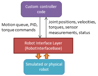
“Controller” is an overloaded term. Most robots involve a hierarchy of controllers, ranging from low level motor controllers and multi-axis Cartesian controllers that run at 100’s of Hz, to sensor feedback logic like visual servoing or obstacle avoidance that run at 10s of Hz, up to motion planning, user interfaces, and mission control which operate at 1 Hz or less. The word “controller” here refers to the lowest level controllers, while slower application-level controllers is referred to as the “application”. Klampt’s Robot Interface Layer is the bridge between the two.

Klamp’t Robot Interface Layer

Starting in version 0.9, Klamp’t Robot Interface Layer (RIL) is fully adopted as Klampt’s preferred method for interfacing with simulated and real robots. RIL is designed to save robot developers a huge amount of time and solve a number of issues in a unified framework:

• Building complex robot controllers from the ground up: given motor drivers and a URDF, RIL utilities will automatically turn any set of servos into a unified robot, with functions available on the most sophisticated motor controllers. Klampt RIL can provide Cartesian control, smooth motion generation, and collision avoidance (by stopping).

• Building Frankenstein robots from multiple parts: multi-component robots with a set of arms, grippers, mobile base, etc. can be built and addressed as a unit. A single line of code will do all the work of gathering state variables, multiplexing commands, and emulating behavior that parts don’t inherently provide.

• Easy switching between sim and real: you’d like to prototype an application in simulation, and after debugging it in sim, switch immediately to a real robot. RIL lets you do switch backends in one line of code.

• Fine grained controller development and debugging: developers can debug exactly how a controller operates, with complete control over step by step operation.

• Procedural application control: building high-level procedural application logic is easy. Just command a motion, call interface.wait(), and continue.

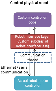
The RIL consists of the main RobotInterfaceBase class, which provides a superset of common functionality that most robots’ motor controllers provide, as well as accessors for custom functionality.

The overall diagram looks like the following:

To interface with your own robot, you will need to subclass RobotInterfaceBase to provide the intended functionality, or find someone else’s implementation for your brand / type of robot.

Writing Control Loops

An RIL API can either be synchronous or asynchronous. Synchronous APIs are a little more fussy, requiring that all commands and queries at a given time step are placed within a beginStep()/endStep() block which is run at approximately a fixed rate. The calling convention is:

interface = MyRobotInterface(...args...)
if not interface.initialize():  #should be called first
    raise RuntimeError("There was some problem initializing interface "+str(interface))
dt = 1.0/interface.controlRate()
status = 'ok
while status == 'ok':  #no error handling done here...
    t0 = time.time()
    interface.beginStep()
    status = interface.status()
    [any interface queries / commands here comprising the control loop]
    interface.endStep()
    t1 = time.time()
    telapsed = t1 - t0
    [wait for time max(dt - telapsed,0)]
interface.close()

To make your code even simpler, we provide the helper classes TimedLooper and StepContext which are used as follows:

from klampt.control import TimedLooper,StepContext

interface = MyRobotInterface(...args...)
if not interface.initialize():  #should be called first
    raise RuntimeError("There was some problem initializing interface "+str(interface))
looper = TimedLooper(dt = 1.0/interface.controlRate())
status = 'ok'
while status == 'ok' and looper:  #no error handling done here...
    with StepContext(interface):
        status = interface.status()
        [any interface queries/ commands here comprising the control loop]
interface.close()

An asynchronous controller is much easier to work with: just initialize, and call whatever queries and commands you wish:

interface = MyRobotInterface(...args...)
if not interface.initialize():  #should be called first
    raise RuntimeError("There was some problem initializing interface "+str(interface))
[any interface queries / commands can go here, for example...]
q = interface.commandedPosition()
q[0] += 0.1
interface.moveToPosition(q)
interface.wait()
q[0] -= 0.1
interface.moveToPosition(q)
interface.wait()
interface.close()

You are free to use the synchronous convention with asynchronous controllers as well.

To determine whether an RIL interface is asynchronous, test interface.properties.get('asynchronous',False).

Status Management

• interface.initialize(): must be called before the control loop. May return False if there was an error connecting.

• interface.status(): returns ‘ok’ if everything is ok. Otherwise, returns an implementation-dependent string.

• interface.clock(): returns the robot’s clock, in s.

• interface.controlRate(): returns the control rate, in Hz.

• interface.reset(): if status() is not ‘ok’, tries to reset to an ok state. A controller should not issue commands until status() is ‘ok’ again.

• interface.estop(): triggers an emergency stop. Default just does a soft stop.

• interface.softStop(): triggers a soft stop.

DOFs, Joints, and Parts

The number of DOFs in RIL is assumed equal to the number of joints with actuators and encoders. If the robot has fewer actuators than encoders, the commands for unactuated joints should just be ignored. If the robot corresponds to a Klampt model (typical), then the number of DOFs should be model.numDrivers().

DOF Accessors

• interface.numJoints(): returns the # of DOFs.

• interface.indices(): returns a list of indices of all the robot’s DOFs (equivalent to list(range(numJoints())).

• interface.indices(joint_idx=j): returns the index of the given DOF index (equivalent to j).

• interface.jointName(j): returns the name of the j’th joint.

A robot can have “parts”, which are named groups of DOFs. For example, a robot with a gripper can have parts “arm” and “gripper”, which can be controlled separately.

Part Accessors

• interface.parts(): retrieves the list of part names.

• interface.indices(part): retrieves the indices of this robot accessed by part part.

• interface.indices(part,j): retrieves the index on this robot accessed by joint j on part part (equivalent to indices(part)[j]).

• interface.partInterface(part): access a RIL interface to a part.

Command types

RIL supports position control, velocity control, torque control, piecewise linear and piecewise cubic interpolation, as well as smooth move-to commands. It also allows Cartesian commands to be configured and issued.

Each of these commands begins immediately and returns to the caller immediately. A command overrides any prior command to the robot.

Keep in mind that almost all robots will only implement a subset of these natively; other commands will be software emulated (via klampt.control.robotinterfaceutils.RobotControllerCompleter). For example, simply implementing setPosition and then completing it will suffice.

Low-level control

• interface.setPosition(q): Immediate position control.

• interface.setVelocity(v,ttl=None): Immediate velocity control, with an optional time-to-live.

• interface.setTorque(t,ttl=None): Torque control, with an optional time-to-live.

• interface.setPID(q,dq,t_feedforward=None): PID command, with optional feedforward torque.

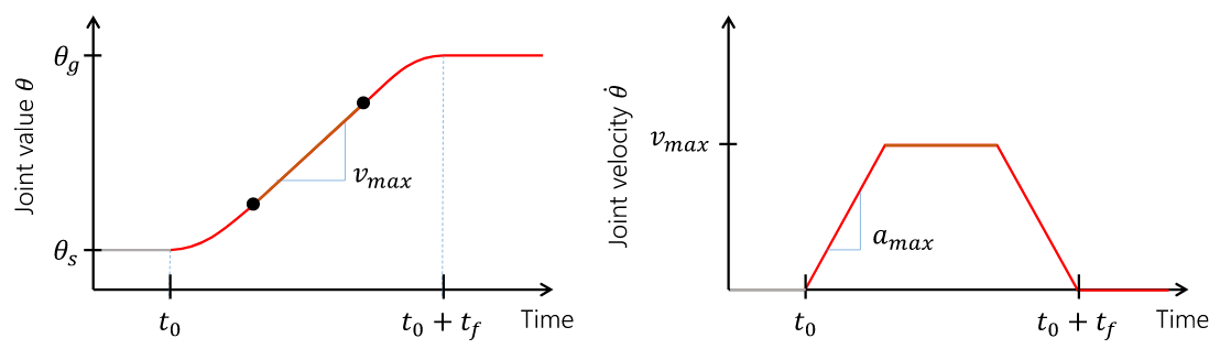
Motion queue control

A motion queue will progressively dole out position, velocity, or PID commands to the underlying joint controllers. A conceptual illustration is as follows.

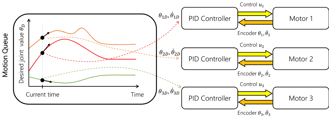
• interface.moveToPosition(q,speed=1): Smooth position control. The semantics of how the motion is generated is implementation-dependent.

• interface.setPiecewiseLinear(times,milestones,relative=True): initiates a piecewise linear trajectory between the given times and milestones. If relative=True, time 0 is the current time, but otherwise all the times should be greater than interface.clock().

• interface.setPiecewiseCubic(times,milestones,velocities,relative=True): initiates a piecewise cubic trajectory between the given times, milestones, and velocities. If relative=True, time 0 is the current time, but otherwise all the times should be greater than interface.clock().

• interface.destinationConfig(): returns the final configuration of the queue.

• interface.destinationTime(): returns the clock time at which the destination is expected to be reached.

Cartesian control

Each RIL robot has at most one end effector. If you have a robot with multiple end effectors, you will need to create a part for each end effector.

All Cartesian items are specified in some frame, which is by default the world frame defined by the robot. For 6DOF robots, the task space should be SE(3) (klampt.math.se3 element). For 3DOF robots the task space is likely to be 3D.

• interface.setToolCoordinates(x): sets the tool center point

• interface.getToolCoordinates(): gets the tool center point

• interface.setGravityCompensation(gravity=[0,0,-9.8],load=0,load_com=[0,0,0]): sets the gravity compensation vector, load, and load position relative to the base frame of the robot.

• interface.setCartesianPosition(x,frame='world'): sets an immediate position command to the position x.

• interface.moveToCartesianPosition(x,speed=1.0,frame='world'): sets a move-to cartesian command. This is not necessarily a straight line motion. (TODO: if the base moves, this might not end up at the right position!)

• interface.moveToCartesianPositionLinear(x,speed=1.0,frame='world'): sets a move-to cartesian command, moving in a straight line

• interface.setCartesianVelocity(dx,ttl=None,frame='world'): sets an immediate velocity command with the task space velocity dx. For an SE(3) task space, dx=(w,v) with w the angular velocity and v is the translational velocity.

• interface.setCartesianForce(fparams,ttl=None,frame='world'): sets a Cartesian force command. For an SE(3) task space, fparams=(torque,force) gives the wrench acting on the end effector.

For most robots, frame=’world’ is equivalent to frame=’base’. For sub-robots, frame=’base’ is measured with respect to the robot’s base. When the robot’s base might move, such as a mobile manipulator, frame=’world’ moves the target while tracking the commanded base frame, which will do the “right thing” in world coordinates. ‘tool’ and ‘end effector’ are also possible frames (Note: these are not tested very thoroughly at the moment).

Controlling Simulated Robots

It’s extremely useful to test your application in simulation so that it can work directly when you switch to the real robot. To do so, Klamp’t provides classes in klampt.control.simrobotinterface that allow you to bind your robot to Klampt simulations.

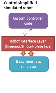
You should pick the RIL interface that corresponds most closely to your actual robot, whether it’s position controlled, velocity controlled, or provides motion queue functionality. SimXControllInterface classes are available to use physics simulation as well as basic kinematic simulation (KinematicSimControlInterface), which is faster. This usage is summarized in the following diagrams.

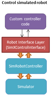
Note that underlying the physics simulation are the simulated robot controller SimRobotController and sensor SimRobotSensor classes. To configure the behavior of the simulated motors and sensors, see Robot Controllers in Simulation, the simulation documentation, and the sensor documentation.

Controller File Format

RIL interfaces are specified to most tools in a standardized controller file format, specifically, a .py file or python module with a single make(robot) function that returns a subclass of RobotInterfaceBase. For example, klampt.control.simrobotcontroller returns a kinematically simulated robot interface. Several example controller files for UR5 robots, Robotiq grippers, and the Kinova Gen 3 are given in Klampt-examples/robotinfo.

This file format is used by klampt_control and RobotInfo, and we plan for it to be the method by which we refer to controller code in the future.

Implementing RIL for Your Robot

To implement an RIL layer for your robot, you will need to understand details on the communication method used by the manufacturer, e.g., Ethernet, serial, ROS, or some other API. Your RIL implementation should fill out as much of the RobotInterfaceBase methods as provided by the communication layer. The block diagram of the architecture looks like this:

For RIL to work, there are a few functions your subclass will need to fill out, at a minimum:

• numJoints(), klamptModel(), or properties['klamptModelFile'].

• Either controlRate() or clock()

• Either setPosition(), moveToPosition(), setVelocity(), setTorque(), or setPID()

• Either sensedPosition() or commandedPosition()

Given these implementations, we provide a convenience class, RobotInterfaceCompleter, that will automatically fill in all other parts of the RIL API, e.g., velocity control, motion queue control, and Cartesian control.

Below is a minimal RIL template, including the standard make function that is required for standard RIL controller files:

from klampt.control import RobotInterfaceBase,RobotInterfaceCompleter

class MyRobotDriver(RobotInterfaceBase):
    def __init__(self):
        RobotInterfaceBase.__init__(self)
        self.properties['klamptModelFile'] = 'path/to/my/URDF'

    def initialize(self):
        #TODO: connect to robot
        return True

    def controlRate(self):
        return 10  #10Hz or whatever

    def setPosition(self,q):
        #TODO: send a position command
        raise NotImplementedError()

    def sensedPosition(self):
        #TODO: return current joint positions
        raise NotImplementedError()

def make(robotModel):
    return RobotInterfaceCompleter(MyRobotDriver())

Place this in myrobot.py and run klampt_control myrobot.py. That’s it!

Note

Move-to and Cartesian control functions are only available if RobotInterfaceBase.klamptModel() is implemented.)

Software Emulation

The RobotControllerCompleter class will perform software-based motion generation, Cartesian control, and filtering automatically given a base interface that implements at least one low-level command, such as setPosition. It can also create virtual parts, mixing-and-matching medium-level control (e.g., an arm cartesian command) and low-level control (e.g., a gripper setVelocity command) seamlessly.

For motion generation during moveToPosition and moveToCartesianPosition commands, the emulator will compute time-optimal acceleration-bounded trajectories. For this to work well, it is very important that the klamptModel() have accurate velocity and acceleration bounds.

To enable Cartesian control, you will need to call addPart to create a part whose last index corresponds to the driver in klamptModel() whose link matches the end effector. Then, retrieve the part interface via partInterface(partName) and call setToolCoordinates([toolx,tooly,toolz]).

Frankenstein Robots

We often build robots out of several components, such as an arm and a gripper, and it can be a pain to coordinate the control of each component. Klamp’t provides a convenience class, OmniRobotInterface, that lets you assemble robots into parts.

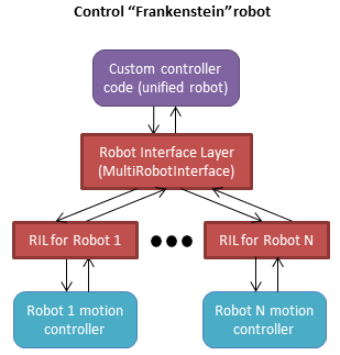
OmniRobotInterface handles software emulation of all methods, similar to RobotInterfaceCompleter. It can also add virtual parts, such as the arm part of a 6+1 robot with arm and gripper, so that Cartesian control can be used.

Limit, Collision, and Sensor Filters

Implementers will also want to figure out how joint limit and collision handling are implemented. You may also add “server side” signal processing for filtering sensor signals. To do this, we have the notion of a filter. Implementers will add desired filters on their RobotInterfaceCompleter or OmniRobotInterface. They may also do this for any partInterface that you would like commands filtered.

Filters are added using setFilter, but also setJointLimits and setCollisionFilter will automatically configure joint limits and self-collisions / obstacle collisions.

Asynchronous Interfaces

The best practice for implementing an RIL API is to use an asynchronous interface that does not require the caller to operate with the device driver in lock-step.

Automagic method: The ThreadedRobotInterface and MultiprocessingRobotInterface classes build asynchronous . Wrapping a synchronous controller, e.g., ThreadedRobotInterface(MyInterface()), will generate an asynchronous interface. Note that beginStep() and endStep() do not need to called in asynchronous mode.

Manual method: To make your own threaded implementation, you should launch a thread that synchrononously communicates with your robot, while relaying asynchronous commands from the caller. The following code does a very basic job of this for a position-controlled robot, which only relays the sensed/ commanded positions to/from the robot.

from klampt.control.robotinterface import *
from klampt import *
from threading import Thread,Lock

class RobotCommThread:
  def __init__(self,connection):
    Thread.__init__(self)
    self.connection = connection
    self.doStop = False
    self.lock = Lock()
    self.commandedPosition = None
    self.sensedPosition = None
    self.new_commandedPosition = None
    self.status = 'ok'
    self.daemon = True  #flag in Thread that will help kill this Thread under Ctrl+C
  def run(self):
    while not self.doStop:
      with self.lock:
        ...read status, sensedPosition, commandedPosition from the robot...
        ...if disconnected, set status to 'disconnected'...
        if self.new_commandedPosition is not None:
          ...send new_commandedPosition to the robot...
          self.commandedPosition = new_commandedPosition
      #unlock
      time.sleep(0.001) # or some small amount

class MyRIL(RobotInterfaceBase):
  def __init__(self):
    RobotInterfaceBase.__init__(self)
    self.thread = None
    self.world = WorldModel()
    self.world.readFile(...path to robot file...)
    self.robot = self.world.robot(0)
    self.properties['asynchronous'] = True
  def initialize(self):
    ...connect to the robot, return False if unsuccessful...
    self.thread = RobotCommThread(robot_connection)
    self.thread.start()
  def stop(self):
    if self.thread is not None:
      self.thread.doStop = True
      self.thread.join()
      self.thread = True
  def klamptModel(self):
    return self.robot
  def controlRate(self):
    return ...whatever the robot's control rate is...
  def status(self):
    return self.thread.status
  def commandedPosition(self):
    with self.thread.lock:
      return self.thread.commandedPosition
  def sensedPosition(self):
    with self.thread.lock:
      return self.thread.sensedPosition
  def setPosition(self,q):
    with self.thread.lock:
      self.thread.new_commandedPosition = q

(Note: a complete implementation will do a better job of error handling.)

ROS Implementations

For a ROS implementation, ROS messaging will already be running in a separate thread, so you don’t need to set up a new thread after you’ve run rospy.init_node(...). This could happen, for example, in the initialize method. Then, for all robot commands provided by your robot’s ROS interface:

1. In the appropriate RIL method, translate the Klamp’t command to a ROS message.

2. Publish the message to the appropriate topic, or call the appropriate service.

For all sensor messages provided by your robot’s ROS interface:

1. In initialize, set up a subscriber to the sensor message.

2. The callback from that subscriber should just store the sensor message.

3. Overload the appropriate RIL method to translate the ROS message to a Klamp’t object. For standard positions, velocities, and torques, use the sensedPosition(), sensedVelocity(), and sensedTorque() methods.

   For more complex, asynchronous items like laser sensors, cameras, RGB-D sensors, and force/torque sensors, you should use the sensors(), sensorMeasurements(), and sensorUpdateTime() methods. For best interpretability (and compatibility with Klampt’s visualization tools, e.g. RobotInterfacetoVis), you should also make sure the sensor is defined in the robot’s klamptModel() model, and that these measurements match the format of the corresponding Klamp’t sensor.

As an example, consult the implementation of RosRobotInterface. This class sends ROS JointTrajectory commands and receives ROS JointState sensor messages.

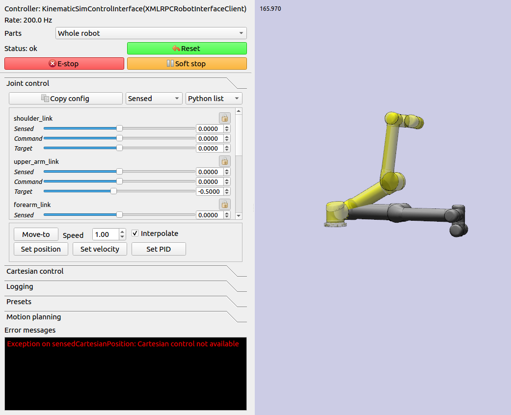
Klampt Control App

The klampt_control app helps debug functionality of RIL interfaces. It allows you to pose the robot, set joint and Cartesian targets, and control individual parts as well. Moreover, it offers a standard server/client interface to your RIL controllers.

klampt_control allows you to operate robots in real time, to debug implementations of Robot Interface Layer (RIL) controllers, and launch RIL controllers in server or client mode.

A controller script is a Python file or module that contains a function make(RobotModel) -> RobotInterfaceBase. We recommend including such a script in a RobotInfo JSON file, which specifies the controller, model, parts, and end effectors:

klampt_control Klampt-examples/robotinfo/ur5/ur5_sim.py

Alternatively, the script may be specified directly on the command line along with the associated robot or world model. The following launches an interface to control a physical UR5 robot:

klampt_control Klampt-examples/robotinfo/ur5/controller/ur5_ril.py Klampt-examples/data/robots/ur5.rob

The default kinematic simulation interface is specified with klampt.control.simrobotcontroller, so the following controls a virtual UR5:

klampt_control klampt.control.simrobotcontroller Klampt-examples/data/robots/ur5.rob

Similarly, you can just include the --sim flag:

klampt_control --sim Klampt-examples/data/robots/ur5.rob

To launch a controller as an XML-RPC server, you can simply pass the --server flag:

klampt_control --server 0.0.0.0:7881 Klampt-examples/robotinfo/ur5/ur5_sim.rob

To run the klampt_control GUI in client mode, run:

klampt_control --client http://localhost:7881

If you are not running on the same machine or do not have the same directory structure, you will need to specify the robot file as well:

klampt_control --client http://[SERVER_IP]:7881 Klampt-examples/robotinfo/ur5/ur5_sim.rob

Note: klampt_control currently does not support logging or motion planning, but will do so in a future version of Klampt.

Under the Hood

Robot Controllers in Simulation

Most users will want to write their application logic using the RIL interfaces in the klampt.control.simrobotcontroller module, because these permit easily switching to a real robot controller. However, implementers of robot simulations will need to know how robot controllers are simulated more deeply.

The overall structure of a simulated robot controller is shown below. The Python wrappers for the simulated items are in the SimRobotController and SimRobotSensor classes.

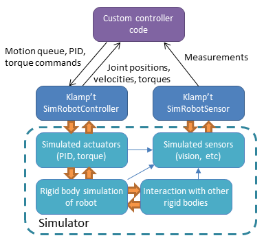
Actuators

At the lowest level, a robot is driven by forces coming from actuators. These receive instructions from the controller and produce link torques that are used by the simulator. Klamp’t simulators support two types of actuator:

• Torque control accepts torques and feeds them directly to links.

• PID control accepts a desired joint value and velocity and uses a PID control loop to compute link torques servo to the desired position. Gain constants kP, kI, and kD should be tuned for behavior similar to those of the physical robot. PID controllers may also accept feedforward torques.

Note that PID control is performed as fast as possible with the simulation time step. This rate is typically faster than that of the calling controller. Hence a PID controlled actuator typically performs better (rejects disturbances faster, is less prone to instability) than a torque controlled actuator with a simulated PID loop at the controller level.

Important

When using Klamp’t to prototype behaviors for a physical robot, the simulated actuators should be calibrated to mimic the robot’s true low-level motor behavior as closely as possible. It is also the responsibility of the user to ensure that the controller uses the simulated actuators in the same fashion as it would use the robot’s physical actuators. For example, for a PID controlled robot with no feedforward torque capabilities, it would not be appropriate to use torque control in Klamp’t. If a robot does not allow changing the PID gains, then it would not be appropriate to do so in Klamp’t. Klamp’t will not automatically configure your controller for compatibility with the physical actuators, nor will it complain if such errors are made.

Default Motion Queue Controller

The default SimRobotController for simulated robots is a motion-queued controller with optional feedforward torques, which simulates typical controllers for industrial robots. The trajectory interpolation profile is the standard trapezoidal velocity profile, except it also accepts interruption and arbitrary start and goal velocities.

(Note: One limitation of the API is that it is impossible to have a subset of joints controlled by a motion queue, while others are controlled by PID or torque commands.)

API summary

Basic commands

• controller = sim.getController(RobotModel or robot index): retrieves the simulation controller for the given wobot

• controller.setPIDGains (kP,kI,kD): overrides the PID gains in the RobotModel to kP,kI,kD (lists of floats of lengths robot.numDrivers())

• controller.setRate(dt): sets the time step of the internal controller to update every dt seconds

• controller.setPIDCommand(qdes,[dqes]): sets the desired PID setpoint

• controller.setVelocity(dqdes,duration): sets a linearly increasing PID setpoint for all joints, starting at the current setpoint, and slopes in the list dqdes. After duration time it will stop.

• controller.setTorque(t): sets a constant torque command t, which is a list of n floats.

Motion queue operations (wraps around a PID controller)

Convention: setX methods move immediately to the indicated milestone, add/append creates a motion from the end of the motion queue to the indicated milestone

• controller.remainingTime(): returns the remaining time in the motion queue, in seconds.

• controller.set/addMilestone(qdes,[dqdes]): sets/appends a smooth motion to the configuration qdes, ending with optional joint velocities dqdes.

• controller.addMilestoneLinear(qdes): same as addMilestone, except the motion is constrained to a linear joint space path (Note: addMilestone may deviate)

• controller.set/appendLinear(qdes,dt): sets/appends a linear interpolation to the destination qdes, finishing in dt seconds

• controller.set/addCubic(qdes,dqdes,dt): moves immediately along a smooth cubic path to the destination qdes with velocity dqdes, finishing in dt seconds

Querying robot state

• controller.getCommandedConfig(): retrieve PID setpoint

• controller.getCommandedVelocity(): retrieve PID desired velocity

• controller.getSensedConfig(): retrieve sensed configuration from joint encoders

• controller.getSensedVelocity(): retrieve sensed velocity from joint encoders

• controller.sensor(index or name): retrieve SimRobotSensor reference by index/name

Emulating Cartesian Control

The Cartesian velocity control emulator used by RobotInterfaceCompleter uses the CartesianDriveSolver class. This may be handy for some controller implementations, but most users will just want to use RobotInterfaceCompleter.

Its drive() method is called repeatedly to incrementally drive the end effector (or end effectors) along desired translational and angular velocities. At each time step, a precise Cartesian motion (a screw motion) is executed, where possible.

CartesianDriveSolver is better than using an IK solver to solve for each velocity increment, because the errors of an IK solver will accumulate, causing a drift from the desired motion. Instead, the solver maintains a Cartesian “marker” that designates the desired pose, and its position is incremented via integration along the desired screw motion. (There may be slight numerical errors due to the limits of machine precision, but they will be imperceptable even at sub-millimeter resolutions.)

Some Cartesian velocities are not possible due to joint limits, velocity limits, and kinematic constraints. If a non-realizable velocity is commanded, then the solver moves the marker as far as possible along the commanded screw motion. Future commands will drive the marker from whatever pose was achieved. This means the robot can recover from being driven to singularities by driving the marker back toward the reachable space. (Note that it can still be challenging to recover from joint limits, since the fraction of directions that lead back to the reachable set is reduced by each constraint met.)

The usage pattern with a simulated robot is as follows:

import klampt
from klampt.control.cartesian_drive import CartesianDriveSolver

world = klampt.WorldModel()
world.readFile("my_world_file.xml")
robot = world.robot(0)
sim = klampt.Simulator(world)
controller = sim.controller(0)

#configure the solver
driver = CartesianDriveSolver(robot)
ee_link = robot.numLinks()-1  #what's the end effector link?
tool_position = [0,0,0]   #local position of the tool center point on the end effector
driver.start(controller.getCommandedConfig(),ee_link,endEffectorPositions=tool_position)

#begin the loop
dt = 0.01
while sim.getTime() < 10:
    #TODO put your control code here
    q = controller.getCommandedConfig()
    ang_vel = [0,0,0]      #angular velocity
    lin_vel = [0.1,0,0]    #lin_vel
    (progress,qnext) = driver.drive(q,ang_vel,lin_vel,dt)
    controlller.setPIDCommand(qnext,[0]*len(q))
    if progress < 0:
        print("Progress stopped?")

    #advance the simulation
    sim.simulate(dt)
print("End configuration:",controller.getSensedConfig())

This approach is local, and does not verify whether a path is executable or not. Another approach to Cartesian control is to convert from a Cartesian path to a joint-space path using the utilities in cartesian_trajectory. Straight-line paths can be executed using cartesian_move_to(). For example, this code generates a linear Cartesian path (0.25m forward in the X direction) that can be executed by joint-space motions:

from klampt.model.cartesian_trajectory import cartesian_move_to
from klampt.model.trajectory import path_to_trajectory,execute_trajectory
from klampt.model import config,ik
from klampt.math import vectorops

...setup world, robot, and controller as before

# Now we set up a target
ee_link = robot.numLinks()-1
T0 = robot.link(ee_link).getTransform()
goal = ik.objective(robot.link(ee_link),R=T0[0],t=vectorops.add(T0[1],[0.25,0,0]))
# Calling this function will generate a path from the current e.e. transform to goal
path = cartesian_move_to(robot,goal)
if path is None:
    print("Couldn't find a path!")
else:
    # Now the path can be executed on a controller... note that it's untimed,
    # so a little work needs to be done to make it timed.  The path_to_trajectory
    # utility function helps a lot here!  It has many options so please consult
    # the documentation...
    traj = path_to_trajectory(path,smoothing=None,timing='Linf')
    speed = 1.0   #can vary the execution speed here or in path_to_trajectory.
    execute_trajectory(traj,controller,speed=speed)

while sim.getTime() < 10:
    #advance the simulation
    sim.simulate(dt)

Importantly, the feasibilityTest argument can be used to verify constraints, such as self collision:

def feasibilityTest(q):
    robot.setConfig(q)
    return not robot.selfCollision()
path = cartesian_move_to(robot,goal,feasibilityTest=feasibilityTest)

See the Paths and Trajectories manual for more detail about the path_to_trajectory() and execute_trajectory() functions.

System Building Blocks

A Block interface is a very simple object with two important methods:

• advance(self,**inputs): given a set of inputs, produce a set of outputs. The semantics of the inputs and outputs are defined by block initializer. The block moves forward single time step, performing any necessary changes to internal state.

• signal(self,type,**inputs): sends some asynchronous signal to the controller. The usage is caller dependent.

Optionally, it can also implement __getstate__/__setstate__.

Robot controller blocks

A Block that operates as the top-level controller for a robot is said to follow the RobotControllerBlock convention. The input dictionary contains sensor messages, specifically containing the following elements:

• t: the current simulation time

• dt: the controller time step

• q: the robot’s current sensed configuration

• dq: the robot’s current sensed velocity

• The names of each sensors in the simulated robot controller, mapped to a list of its measurements.

The RobotControllerBlock output dictionary represents a command message. to be sent to the robot’s low-level motor controllers. A command message can have one of the following combinations of keys, signifying which type of joint control should be used:

• qcmd: use PI control.

• qcmd and dqcmd: use PID control.

• qcmd, dqcmd, and torquecmd: use PID control with feedforward torques.

• dqcmd and tcmd: perform velocity control with the given actuator velocities, executed for time tcmd.

• torquecmd: use torque control.

The klampt_sim script accepts arbitrary feedback controllers in this form. To specify such a controller, provide as input a .py file with a single make(robot) function that returns a subclass of RobotControllerBlock that implements the desired functionality. For example, to see a controller that interfaces with ROS, see klampt/control/io/roscontroller.py.

Building controllers from blocks

Internally the controller can produce arbitrarily complex behavior. Several common blocks are implemented in klampt.control.blocks.

• TimedControllerSequence: runs a sequence of sub-controllers, switching at predefined times.

• MultiController: runs several sub-controllers in parallel, with the output of one sub-controller cascading into the input of another. For example, a state estimator could produce a better state estimate q for another controller.

• ComposeController: composes several sub-vectors in the input into a single vector in the output. Most often used as the last stage of a MultiController when several parts of the body are controlled with different sub-controllers.

• LinearBlock: outputs a linear function of some number of inputs.

• LambdaBlock: outputs f(arg1,...,argk) for any arbitrary Python function f.

• StateMachine: a base class for a finite state machine controller. The subclass must determine when to transition between sub-controllers.

• TransitionStateMachine: a finite state machine controller with an explicit matrix of transition conditions.

A trajectory tracking controller is given in klampt/control/blocks/trajectory_tracking.py. Its make function accepts a robot model (optionally None) and a linear path file name.

A preliminary velocity-based operational space controller is implemented in control-examples/OperationalSpaceController.py, but its use is highly experimental at the moment.

State estimation

State estimators can be implemented as Block subclasses that calculate the estimated state objects in the advance() method.