Inverse Kinematics
There are two components that need to be set up to solve inverse kinematics problems.
First, an IK Objective object must to be configure to define constraints on a constrained link.
Next, the IK Solver is set up and called to find a configuration so that the transformations satisfy the constraints specified by the objectives.
Multiple links can be constrained to different targets by creating several IK Objectives and passing these to the solver.
IK Objective
An IK Objective defines a target in Cartesian world space coordinates that you want to achieve with a link of the robot. Each IK Objective’s constraint specifies “I desire that” some local coordinates on the link should be matched to some target coordinates. These coordinates may include both position and orientation.
An objective contains:
A link index
A rotation constraint type: none, axial, fixed
A position constraint type: none, planar, linear, fixed
For non-none constraints, a local position and a target position
For planar and linear constraints, a direction of the plane/line
For non-none constraints, a target rotation
For axial constraints, a rotation axis
Klamp’t also supports relative IK Objectives that let you define a constraint from coordinates on one link relative to another on the same robot, but these are used less frequently. The main use case for these objectives is to perform multi-handed manipulation of a single object. Relative objectives are specified by giving:
an index of a destination link. (By default the destination link is -1, which means the targets are specified in the world frame.)
Usual Objective Types
Constraint type |
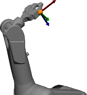
Point |
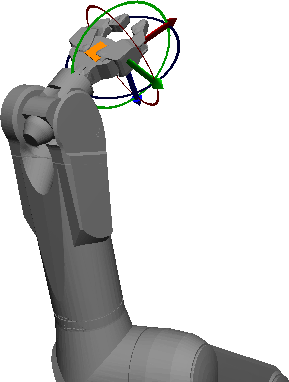
Fixed |
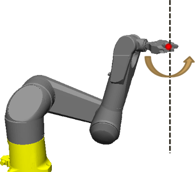
Hinge |
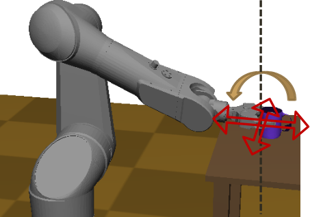
Surface |
|---|---|---|---|---|
Position |
fixed |
fixed |
fixed |
planar |
Rotation |
none |
fixed |
axis |
axis |
Constrained dims |
3 |
6 |
5 |
3 |
Useful for |
Point feet or fingers |
Grasps, flat feet |
Grasping cylindrical objects |
Placing objects down with unspecified position and orientation |
|
|
|
|
The SimTest and RobotPose programs only support point and fixed constraint types. More exotic types must be created in code.
API summary
The core functionality is contained in the
IKObjective
class, but there are more convenient methods in
the klampt.model.ik
module. The following assume that you have first run
from klampt import IKObjective,IKSolver
from klampt.model import ik
Constructors
obj = ik.objective(body, ref=None, local=lplist, world=wplist): creates anIKObjectivethat constrains some local points on body (usually a RobotModelLink) to world points. lplist is either a single 3d point or a list of 3d points. wplist taks the same format as lplist, and if it is a list of points, it needs to be of the same length.obj = ik.objective(body, ref=None, R=R, t=t): creates anIKObjectivethat constrains a body (usually aRobotModelLink) so its frame has a fixed rotation R and translation t.obj = IKObjective(): manual constructorobj.setFixedPoint(link,lp,wp): creates a point constraint on the link indexed by link. lp and wp are the 3D local and world points.obj.setFixedPoints(link,lplist,wplist): creates a point constraint on the link indexed by link. lplist and wplist are lists of local and world points.obj.setFixedTransform(link,R,t): creates a fixed constraint on the link indexed by link so its frame has the fixed rotation R and translation t.
Accessors
obj.num[Pos/Rot]Dims(): returns the number of positions of position / orientation constrained (0-3)obj.getPosition(): returns a pair (local,world) of the constrained position. For fixed constraints local is the origin [0,0,0] and world is the target point.obj.getPositionDirection(): if the position has a planar constraint (numPosDims()=1), the normal direction of the plane. If this is an linear constraint (numPosDims()=2), the direction of the lineobj.getRotation(): if the rotation is fixed (numRotDims()=3), the rotation matrix R.obj.getRotationAxis(): if the rotation is axial (numRotDims()=2) returns a pair (laxis,waxis) giving the local / world coordinates of the constrained axis.obj.getTransform(): if this is a fixed constraint, returns the pair (R,t) giving the fixed transform of the link
Convenience methods
obj = ik.fixed_objective(body, ref=None, local=None, world=None): creates an IKObjective that fixes the RobotModelLink in its current location and orientation.obj = ik.fixed_objective(body, ref=None, local=lp, world=None): creates an IKObjective that fixes the local point lp on the RobotModelLink in its current location.obj = ik.fixed_objective(body, ref=None, local=None, world=wp): creates an IKObjective that fixes the world point wp on the RobotModelLink in its current location.obj = ik.fixed_rotation_objective(body, ref=None, local_axis=None, local_axis=None): creates an IKObjective that fixes the RobotModelLink in its current orientation.
Setting up objectives
To set up a point constraint, you will simply fix a local position on the link
localpt to a position in the world worldpt.
from klampt.model import ik
obj = ik.objective(robotlink,local=localpt,world=worldpt)
If this does not give you what you desire, you may wish to use Klampt’s visual editing functionality to debug the local and world points, as follows.
from klampt.io import resource
(save,value) = resource.edit("Local point",localpt,type="Point",frame=robotlink)
if save:
    localpt = value
(save,value) = resource.edit("World point",worldpt,type="Point",frame=None)
if save:
    worldpt = value
obj = ik.objective(robotlink,local=localpt,world=worldpt)
To set up a fixed constraint, you can either use
klampt.model.ik.objective(robotlink,R=link_orientation,t=link_translation)
or set up three non-colinear points that should be constrained from the local frame to three non-colinear points in the world frame.
klampt.model.ik.objective(robotlink,local=[p1,p2,p3],world=[q1,q2,q3])
Note that p1 is constrained to q1, p2 is constrained to q2, etc. Hence, the
distances between each pair of points in p1,p2,p3 must be equal to the
distances between each corresponding pair of points in q1,q2,q3.
To set up a hinge constraint, you can easily set up two points p1,p2 in the local
frame that need to be constrained to two points q1,q2 in the world frame:
ik.objective(robotlink,local=[p1,p2],world=[q1,q2])
To set up a surface constraint, you will need to interact with the IKObjective
class more carefully.
#supposes linkindex, localpt, localaxis, point_on_plane, and plane_normal are given
from klampt import IKObjective
from klampt.math import vectorops
obj = IKObjective()
obj.setLinks(linkindex)
obj.setPlanarPosConstraint(localpt,plane_normal,vectorops.dot(point_on_plane,plane_normal))
obj.setAxialRotConstraint(localaxis,plane_normal)
IK Solver
Klamp’t contains a numerical IK solver, which is extremely flexible and can solve for arbitrary combinations of IK constraints. It takes the robot’s current configuration as a starting point and runs a descent technique to (hopefully) solve all constraints simultaneously.
The solver also can accept optional joint limits and subsets of active DOFs.
Input:
Robot model
One or more IK objectives
Seed configuration is given as the model’s current configuration
Tolerance on max constraint error
Maximum iteration count Optional input:
sub-select active DOFs (default uses all ancestors of constrained links)
custom joint limits
“bias configuration” for redundant robots
Output:
Success or failure (i.e. did not achieve desired tolerance)
Solution configuration is returned inside Robot Model
Specifically, the solver performs Newton-Raphson root solving, with line search (never diverges). These routines automatically try to optimize only over the relevant variables, e.g., if the only constraint is on the robot’s right foot, then the arms, head, and left leg will not be included as optimization variables.
Important
To use the solver properly, you must understand how the solver uses the RobotModel:
First, the current configuration of the robot is the seed configuration to the solver.
Second, the robot’s joint limits are used as the defaults.
Third, the solved configuration is stored in the RobotModel’s current configuration.
IK solvers can also be queried for the IK constraint residual and the constraint Jacobian. These stack the constraint errors of each objective, and can help you debug whether the solver has successfully converged, or whether your objectives were defined incorrectly.
API summary
The solver code is contained in the
IKSolver class, but there are more convenient methods in
the klampt.model.ik
module.
ik.solve(objectives,iters=1000,tol=1e-3,activeDofs=None): Solves one or more IK objectives with the given max iteration count iters and constraint tolerance tol. Returns True if successful. Seeded by the robot’s current configuration, and on output the robot is set to the best found configuration. A list of active DOFs can be provided.solver = ik.solver(objectives): creates a solver for the given (one or more) objectives.solver = IKSolver(robot): creates a solver for the given robot model.solver.add(objective): adds another IKObjective to the solver.solver.setActiveDofs(dofs): sets the active DOFs, given as a list of integer indices (default: all ancestor links of the constrained links).solver.getActiveDofs(): gets the active DOFs as a list of integer indices.solver.setJointLimits(qmin,qmax): sets custom joint limits, each a list of NL limits (default: solver uses the robot model’s joint limits).solver.sampleInitial(): generates a random configuration as the seed.solver.get/setMaxIters(iters): gets/sets the maximum number of iterations allowed per solve call.solver.get/setTolerance(tol): gets/sets the convergence tolerance for the solver (default 1e-3).solver.solve(): solves for the current set of IK objectives and iteration / tolerance settings. Returns True if successful.solver.lastSolveIters(): returns the number of iterations used in the last solve() call.solver.getJacobian()/ik.jacobian(objectives): returns the matrix of IK objective derivatives with respect to the active DOFs.solver.getResidual()/ik.residual(objectives): returns the vector of IK objective values at the robot’s current configuration.
Convenience functions:
-
ik.solve_global(objectives, iters=1000, tol=1e-3, activeDofs=None,
             numRestarts = 100, feasibilityCheck = None, startRandom = False )
Solves one or more IK objectives in a global manner with a random-restart technique. The first 4 arguments are the same as ik.solve. numRestarts gives the number of total restarts attempted before failure is declared. If feasibilityCheck is given, it is a zero-argument function that returns True if the robot’s current configuration is feasible. If startRandom = True, then the robot’s configuration is randomized on the first iteration.
-
ik.solve_nearby(objectives, maxDeviation,
             iters=1000, tol=1e-3, activeDofs=None,
             numRestarts = 0, feasibilityCheck = None )
Solves one or more IK objectives while preventing the robot’s current configuration from deviating more than maxDeviation along each axis.
Example
Find a configuration where the end effector of a planar 3R robot touches the point (1.5,0,1). Let us start doing this in a naive manner:
>>> import klampt
>>> from klampt.model import ik
>>> world = klampt.WorldModel()
>>> world.loadElement("data/robots/planar3R.rob")
...
>>> robot= world.robot(0)
>>> link = robot.link(2)
>>> print(robot.getConfig())
[0.0, 0.0, 0.0]
>>> obj = ik.objective(link,local=[1,0,0],world=[1.5,0,1])
>>> solver = ik.solver(obj)
>>> solver.solve()
False
>>> robot.getConfig()
[0.0, 0.0, 4.215773454225064]
>>> print(solver.getResidual())
[0.023547356775342587, 0.0, -0.12079986421507116]
So why did this fail? Well, the joint limits on the robot don’t allow clockwise rotation from the 0 configuration, so the solver fell into a local minimum where the first two joints are at their lower limit. The solver isn’t that smart about the Robot Joint type, which is a spin joint, which should theoretically have no limits. So, one solution is to turn off the limits, like so:
>>> solver.setJointLimits([],[])  #the values [],[] tell the solver to turn off joint limits
>>> robot.setConfig([0,0,0])
>>> solver.solve()
True
>>> print(robot.getConfig())
[6.2210827440574805, 6.275852672978871, 4.263178112891824]
>>> print(solver.getResidual())
[-4.36569416761845e-06, 0.0, -2.3191920574427982e-05]
Another rationale is that the initial seed configuration as not chosen well, and a different choice of initial seed might have led to a global minimum. A simple approach for doing this is is to use random restarts, one iteration of which is shown as follows:
>>> solver.setJointLimits(*robot.getJointLimits())    #reinstantiate joint limits
>>> solver.sampleInitial()   # the initial configuration didn't let the solver find a solution, sample a new one
>>> solver.solve()
True
>>> print(robot.getConfig())
[0.9280844225663805, 5.24982420453923, 2.3118916002271988]
>>> print(solver.getResidual())
[-4.36569416761845e-06, 0.0, -2.3191920574427982e-05]
We can visualize the result as follows:
>>> from klampt import vis
>>> vis.add("world",world)    #shows the robot in the solved configuration
>>> vis.add("local point",link.getWorldPosition([1,0,0]))
>>> vis.setAttribute("local point","type","Vector3")  #usually the vis module identifies a Config vs a Vector3, but this robot has exactly 3 links
>>> vis.add("target point",[1.5,0,1])
>>> vis.setAttribute("target point","type","Vector3")
>>> vis.setColor("target point",1,0,0)  #turns the target point red
>>> vis.show()  #this will pop up the visualization window until you close it
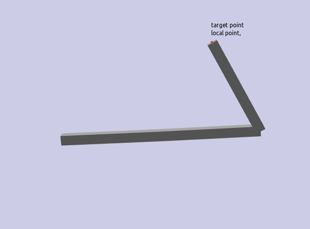
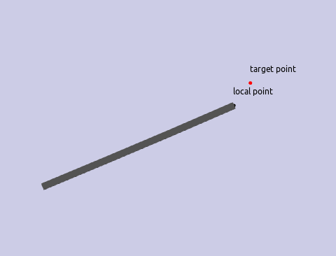
Now suppose we were to change the world position to an unreachable point. The sum of the robot link lengths is 3, so the world position (3,0,1.5) is certainly out of reach. Running the following code, we get that the solver returns False, and the robot is placed at a configuration that reaches almost as close as possible to the target:
>>> obj2 = ik.objective(link,local=[1,0,0],world=[3,0,1.5])
>>> solver = ik.solver(obj2)
>>> solver.setJointLimits([],[])
>>> robot.setConfig([0,0,0])
>>> solver.solve()
False
>>> print(robot.getConfig())
[5.88713697296476, 6.278604588847693, 6.274884577272825]
>>> print(solver.getResidual())
[-0.2390446069453609, 0.0, -0.32659917185852283]
>>> print(link.getWorldPosition([1,0,0]))
[2.760955393054639, 0.0, 1.1734008281414772]
Running the visualization code again, we get something like this:
Exercise
Let us start from Exercise 2 in Klampt-examples/Python3/exercises/ik.
Open up ik.pdf in this folder, and read the instructions. Then run
python ex2.py
to observe the target point animating in a circle. In this exercise we’ll implement the few lines it takes to implement the IK solver.
The end effector link index, local position, and target position in the
world are given to you in this function. Your job is to set up the
structures needed to call the IK solver. Look through ex2.py to find the
place where your code needs to go.
obj = model.ik.objective(robotlink,local=localpos,world=worldpos)
Now we need to 1) set up the solver with the robot and objectives, 2) set the initial configuration to 0 by calling robot.setConfig, and then 3) calling the solver:
s = model.ik.solver(obj)

robotlink.robot().setConfig([0]*robotlink.robot().numLinks())

s.setMaxIters(100)
s.setTolerance(1e-3)
res = s.solve()
numIter = s.lastSolveIters()
if not res: print("IK failure!")
If res=True, then the robot’s configuration is now set to the IK solution. If res=False, then the robot’s configuration is set to the best found configuration.
Alternatively, we could have used a convenience function in klampt.model.ik:
res = model.ik.solve(obj)
if not res: print("IK failure!")
However, note that this will only give you the solution to the IK problem. It will not allow you to later interact directly with the solver. For example, this would mean that you would be unable to access the number of iterations used to obtain an IKSolution.
Either way, though, if all went well, that was pretty simple! Now replace the current return statement with:
return robot.getConfig()
This is done because the IK solver places the resulting configuration in the robot model’s current configuration.
Now run ex2.py again and observe the results.
You can also play around with
the parameters and the start configuration. For example, commenting
out the setConfig line uses the robot’s previous configuration as the
starting point of the optimization. When does this improve the
results? When does this harm them?
Why isn’t IK working?
A common cause of IK failures is local minima. Klamp’t uses a numerical IK solver that iteratively minimizes the error between the current link transform and the goal. It also enforces joint limits. But this iteration can get stuck, most likely due to the joint limits interfering with progress toward the objective. The easiest partial solution for this is to just perform random restarts on the start configuration:
s = ik.solver(obj)

numRestarts = 100
solved = False
for i in range(numRestarts):
        s.sampleInitial()
        s.setMaxIters(100)
        s.setTolerance(1e-3)
        res = s.solve()
        if res:
                solved=True
                break
if not solved: print("IK failure!")
Additionally, Klamp’t has a convenience routine
solve_global() that implements this same functionality in
a single line.
if not ik.solve_global(obj,iters = 100,tol=1e-3,numRestarts=100):
        print("IK failure!")
For feasible objectives, this is likely to come up with a solution in just a few iterations, and not be much more expensive than a single IK solve. But, the increased robustness comes at a price: in the case of infeasible objective, this can take much longer than the standard solver to fail (correctly). By tuning the numRestarts parameter you can trade off between robustness and running time in the case of infeasible objective.
The second likely cause of failures is an incorrectly defined IK objective. The easiest way to debug this is to check the final configuration produced by the IK module. The IK solver does the best it can to satisfy your goal. If it doesn’t appear to be doing what you want, then this is probably an error in defining the objective. Another way is to examine the residual vector, which gives the numerical errors on each of the constrained IK dimensions. To do so, call ik.residual(obj). At a solution, these entries should all be near zero.
Klamp’t also has visualization functionality to display IK objectives.
Simply call visualization.add(name,objective) (you will also want to add
the world) and your constraint will be drawn on screen.
