Control

Controllers provide the “glue” between the physical robot’s actuators, sensors, and planners. Like planners, they generate controls for the robot, but controllers are expected to work online and synchronously within a fixed, small time budget. As a result, they can only perform relatively light computations.

The number of ways in which a robot may be controlled is infinite, and can range from extremely simple methods, e.g., a linear gain, to extremely complex ones, e.g. an operational space controller or a learned policy. Yet, all controllers are structured as a simple callback loop: repeatedly read off sensor data, perform some processing, and write motor commands. The implementation of the internal processing is open to the user.

Simulated Robot Controllers

Note

If you are planning to write a controller that only works in simulation, then continue reading this section. Otherwise, you should skip ahead to the Experimental Robot Interface Layer section to learn how to build controllers that work both in simulation and on real robots.

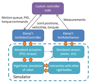
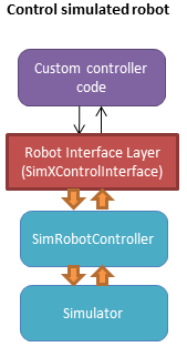
The overall structure of a simulated robot controller is shown below. The primary interfaces to your Python code are in the SimRobotController and SimRobotSensor classes.

Actuators

At the lowest level, a robot is driven by forces coming from actuators. These receive instructions from the controller and produce link torques that are used by the simulator. Klamp’t simulators support two types of actuator:

• Torque control accepts torques and feeds them directly to links.

• PID control accepts a desired joint value and velocity and uses a PID control loop to compute link torques servo to the desired position. Gain constants kP, kI, and kD should be tuned for behavior similar to those of the physical robot. PID controllers may also accept feedforward torques.

Note that PID control is performed as fast as possible with the simulation time step. This rate is typically faster than that of the robot controller. Hence a PID controlled actuator typically performs better (rejects disturbances faster, is less prone to instability) than a torque controlled actuator with a simulated PID loop at the controller level.

Important

When using Klamp’t to prototype behaviors for a physical robot, the simulated actuators should be calibrated to mimic the robot’s true low-level motor behavior as closely as possible. It is also the responsibility of the user to ensure that the controller uses the simulated actuators in the same fashion as it would use the robot’s physical actuators. For example, for a PID controlled robot with no feedforward torque capabilities, it would not be appropriate to use torque control in Klamp’t. If a robot does not allow changing the PID gains, then it would not be appropriate to do so in Klamp’t. Klamp’t will not automatically configure your controller for compatibility with the physical actuators, nor will it complain if such errors are made.

Default Motion Queue Controller

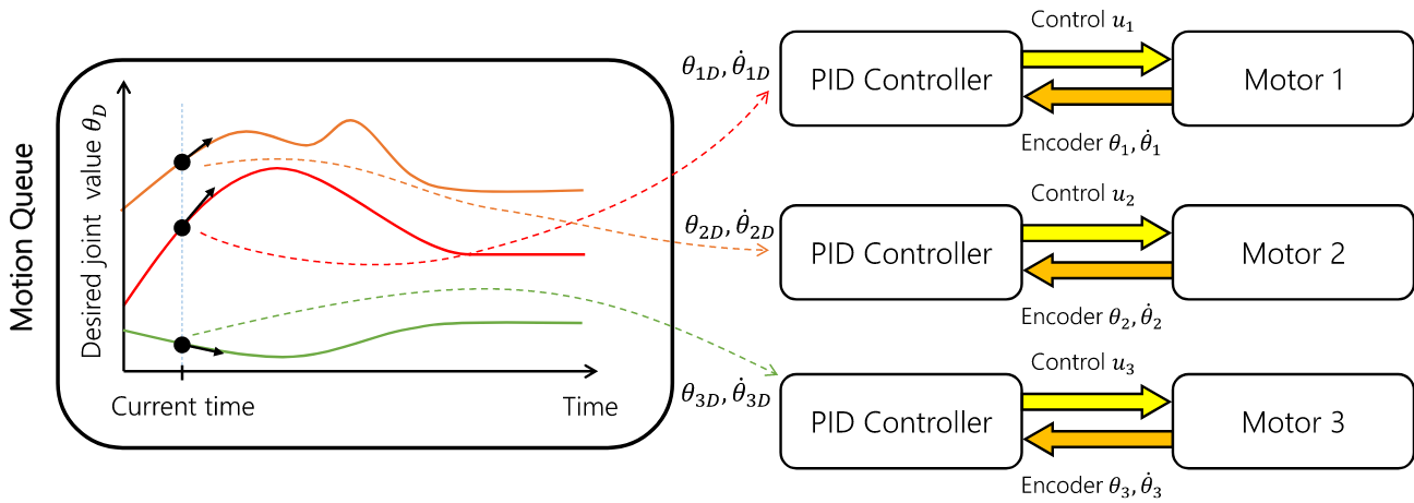
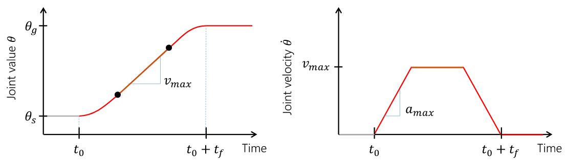
The default SimRobotController for simulated robots is a motion-queued controller with optional feedforward torques, which simulates typical controllers for industrial robots. It supports direct access to actuators, piecewise linear and piecewise cubic interpolation, as well as time-optimal acceleration-bounded trajectories. The trajectory interpolation profile is the standard trapezoidal velocity profile, except it also accepts interruption and arbitrary start and goal velocities.

(Note: One limitation of the API is that it is impossible to have a subset of joints controlled by a motion queue, while others are controlled by PID or torque commands.)

API summary

Basic commands

• controller = sim.getController(RobotModel or robot index): retrieves the simulation controller for the given wobot

• controller.setPIDGains (kP,kI,kD): overrides the PID gains in the RobotModel to kP,kI,kD (lists of floats of lengths robot.numDrivers())

• controller.setRate(dt): sets the time step of the internal controller to update every dt seconds

• controller.setPIDCommand(qdes,[dqes]): sets the desired PID setpoint

• controller.setVelocity(dqdes,duration): sets a linearly increasing PID setpoint for all joints, starting at the current setpoint, and slopes in the list dqdes. After duration time it will stop.

• controller.setTorque(t): sets a constant torque command t, which is a list of n floats.

Motion queue operations (wraps around a PID controller)

Convention: setX methods move immediately to the indicated milestone, add/append creates a motion from the end of the motion queue to the indicated milestone

• controller.remainingTime(): returns the remaining time in the motion queue, in seconds.

• controller.set/addMilestone(qdes,[dqdes]): sets/appends a smooth motion to the configuration qdes, ending with optional joint velocities dqdes.

• controller.addMilestoneLinear(qdes): same as addMilestone, except the motion is constrained to a linear joint space path (Note: addMilestone may deviate)

• controller.set/appendLinear(qdes,dt): sets/appends a linear interpolation to the destination qdes, finishing in dt seconds

• controller.set/addCubic(qdes,dqdes,dt): moves immediately along a smooth cubic path to the destination qdes with velocity dqdes, finishing in dt seconds

Querying robot state

• controller.getCommandedConfig(): retrieve PID setpoint

• controller.getCommandedVelocity(): retrieve PID desired velocity

• controller.getSensedConfig(): retrieve sensed configuration from joint encoders

• controller.getSensedVelocity(): retrieve sensed velocity from joint encoders

• controller.sensor(index or name): retrieve SimRobotSensor reference by index/name

Writing a Custom Controller

To wrap a controller around a simulated robot, the user should implement a control loop. At every time step, the control loop reads the robot’s sensors, computes the control, and then sends the control to the robot via the setPIDCommand or setTorqueCommand methods. You are also free to use the motion queue commands as well. Finally, advance the simulation.

The following example shows a very simple example that just moves the commanded configuration by 1 radian / sec over 10 seconds.

import klampt
world = klampt.WorldModel()
world.readFile("my_world_file.xml")
sim = klampt.Simulator(world)
controller = sim.getController(0)
dt = 0.01
while sim.getTime() < 10:
    #TODO put your control code here
    q = controller.getCommandedConfig()
    q[1] += 1*dt    #move at 1 radian / sec
    controlller.setPIDCommand(q,[0]*len(q))

    #advance the simulation
    sim.simulate(dt)
print("End configuration:",controller.getSensedConfig())

In general, your control loop can make use of sensors and planners. There are countless ways to implement robot behaviors, and you are only limited by your imagination.

Cartesian Control

Smooth Cartesian velocity control can be generated using the CartesianDriveSolver class. Its drive() method is called repeatedly to incrementally drive the end effector (or end effectors) along desired translational and angular velocities. At each time step, a precise Cartesian motion (a screw motion) is executed, where possible.

CartesianDriveSolver is better than using an IK solver to solve for each velocity increment, because the errors of an IK solver will accumulate, causing a drift from the desired motion. Instead, the solver maintains a Cartesian “marker” that designates the desired pose, and its position is incremented via integration along the desired screw motion. (There may be slight numerical errors due to the limits of machine precision, but they will be imperceptable even at sub-millimeter resolutions.)

Some Cartesian velocities are not possible due to joint limits, velocity limits, and kinematic constraints. If a non-realizable velocity is commanded, then the solver moves the marker as far as possible along the commanded screw motion. Future commands will drive the marker from whatever pose was achieved. This means the robot can recover from being driven to singularities by driving the marker back toward the reachable space. (Note that it can still be challenging to recover from joint limits, since the fraction of directions that lead back to the reachable set is reduced by each constraint met.)

The usage pattern with a simulated robot is as follows:

import klampt
from klampt.control.cartesian_drive import CartesianDriveSolver

world = klampt.WorldModel()
world.readFile("my_world_file.xml")
robot = world.robot(0)
sim = klampt.Simulator(world)
controller = sim.controller(0)

#configure the solver
driver = CartesianDriveSolver(robot)
ee_link = robot.numLinks()-1  #what's the end effector link?
tool_position = [0,0,0]   #local position of the tool center point on the end effector
driver.start(controller.getCommandedConfig(),ee_link,endEffectorPositions=tool_position)

#begin the loop
dt = 0.01
while sim.getTime() < 10:
    #TODO put your control code here
    q = controller.getCommandedConfig()
    ang_vel = [0,0,0]      #angular velocity
    lin_vel = [0.1,0,0]    #lin_vel
    (progress,qnext) = driver.drive(q,ang_vel,lin_vel,dt)
    controlller.setPIDCommand(qnext,[0]*len(q))
    if progress < 0:
        print("Progress stopped?")

    #advance the simulation
    sim.simulate(dt)
print("End configuration:",controller.getSensedConfig())

This approach is local, and does not verify whether a path is executable or not. Another approach to Cartesian control is to convert from a Cartesian path to a joint-space path using the utilities in cartesian_trajectory. Straight-line paths can be executed using cartesian_move_to(). For example, this code generates a linear Cartesian path (0.25m forward in the X direction) that can be executed by joint-space motions:

from klampt.model.cartesian_trajectory import cartesian_move_to
from klampt.model.trajectory import path_to_trajectory,execute_trajectory
from klampt.model import config,ik
from klampt.math import vectorops

...setup world, robot, and controller as before

# Now we set up a target
ee_link = robot.numLinks()-1
T0 = robot.link(ee_link).getTransform()
goal = ik.objective(robot.link(ee_link),R=T0[0],t=vectorops.add(T0[1],[0.25,0,0]))
# Calling this function will generate a path from the current e.e. transform to goal
path = cartesian_move_to(robot,goal)
if path is None:
    print("Couldn't find a path!")
else:
    # Now the path can be executed on a controller... note that it's untimed,
    # so a little work needs to be done to make it timed.  The path_to_trajectory
    # utility function helps a lot here!  It has many options so please consult
    # the documentation...
    traj = path_to_trajectory(path,smoothing=None,timing='Linf')
    speed = 1.0   #can vary the execution speed here or in path_to_trajectory.
    execute_trajectory(traj,controller,speed=speed)

while sim.getTime() < 10:
    #advance the simulation
    sim.simulate(dt)

Importantly, the feasibilityTest argument can be used to verify constraints, such as self collision:

def feasibilityTest(q):
    robot.setConfig(q)
    return not robot.selfCollision()
path = cartesian_move_to(robot,goal,feasibilityTest=feasibilityTest)

See the Paths and Trajectories manual for more detail about the path_to_trajectory() and execute_trajectory() functions.

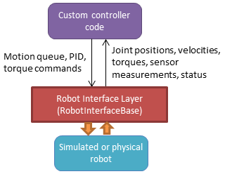
Experimental Robot Interface Layer

Ideally, you’d like to be able to prototype a controller in simulation, and then easily connect the same controller code to a real robot. This is where the Klamp’t Robot Interface Layer (RIL) comes in. The RIL API defines a superset of common functionality that most robots’ motor controllers provide. It also provides a common interface to switch between simulated and real robots. The overall diagram looks like the following:

To interface with your own robot, you will need to construct a subclass of RIL’s main RobotInterfaceBase class, or find someone else’s implementation for your brand / type of robot.

Because creating and debugging such an interface can take some time, it’s useful to test your control code in simulation so that it can work directly when you switch to the real robot. There are two ways to do this:

1. (preferable) Port your control code to use RobotInterfaceBase. Note there are some discrepancies between this and SimRobotController that you should watch out for. Then, use one of the classes in klampt.control.simrobotinterface to test your controller in a simulator.

2. Use your existing control code, but replace your SimRobotController object with a klampt.control.interop.SimRobotControllerToInterface object that points to your robot’s interface.

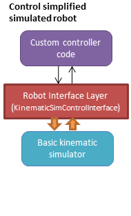
The reason why route 1 is preferable is that you can pick the RIL interface to your simulated robot that corresponds most closely to your actual robot, whether it’s position controlled, velocity controlled, or provides motion queue functionality. SimXControllInterface classes are available to use physics simulation as well as basic kinematic simulation (KinematicSimControlInterface), which is faster. This usage is summarized in the following diagrams.

Using the RIL API

For your controller code to use an RIL API, it should treat the API as a synchronous process, in which all commands and queries at a given time step are placed within a startStep()/endStep() block. The calling convention is:

interface = MyRobotInterface(...args...)
if not interface.initialize():  #should be called first
    raise RuntimeError("There was some problem initializing interface "+str(interface))
dt = 1.0/interface.controlRate()
while interface.status() == 'ok':  #no error handling done here...
    t0 = time.time()
    interface.startStep()
    [any getXXX or setXXX commands here comprising the control loop]
    interface.endStep()
    t1 = time.time()
    telapsed = t1 - t0
    [wait for time max(dt - telapsed,0)]

Status Management

• interface.initialize(): must be called before the control loop. May return False if there was an error connecting.

• interface.status(): returns ‘ok’ if everything is ok. Otherwise, returns an implementation-dependent string.

• interface.clock(): returns the robot’s clock, in s.

• interface.controlRate(): returns the control rate, in Hz.

• interface.reset(): if status() is not ‘ok’, tries to reset to an ok state. A controller should not issue commands until status() is ‘ok’ again.

• interface.estop(): triggers an emergency stop. Default just does a soft stop.

• interface.softStop(): triggers a soft stop.

DOFs, Joints, and Parts

The number of DOFs in RIL is assumed equal to the number of joints with actuators / encoders. If the robot has fewer actuators than encoders, the commands for unactuated joints should just be ignored. If the robot corresponds to a Klampt model (typical), then the number of DOFs should be model.numDrivers().

DOF Accessors

• interface.numJoints(): returns the # of DOFs.

• interface.indices(): returns a list of indices of all the robot’s DOFs (equivalent to list(range(numDOFs())).

• interface.indices(joint_idx=j): returns the index of the given DOF index (equivalent to numDOFs()+j).

• interface.jointName(j): returns the name of the j’th joint.

A robot can have “parts”, which are named groups of DOFs. For example, a robot with a gripper can have parts “arm” and “gripper”, which can be controlled separately.

Part Accessors

• interface.parts(): retrieves the list of part names.

• interface.indices(part): retrieves the indices of this robot accessed by part part.

• interface.indices(part,j): retrieves the index on this robot accessed by joint j on part part.

• interface.partController(part): access a RIL interface to a part.

Command types

Keep in mind that almost all robots will only implement a subset of these natively.

Basic control

• interface.setPosition(q): Immediate position control.

• interface.moveToPosition(q,speed=1): Smooth position control.

• interface.setVelocity(v,ttl=None): Immediate velocity control, with an optional time-to-live.

• interface.setTorque(t,ttl=None): Torque control, with an optional time-to-live.

• interface.setVelocity(v,ttl=None): Immediate velocity control, with an optional time-to-live.

• interface.setPID(q,dq,t_feedforward=None): PID command, with optional feedforward torque.

• interface.setPiecewiseLinear(times,milestones,relative=True): initiates a piecewise linear trajectory between the given times and milestones. If relative=True, time 0 is the current time, but otherwise all the times should be greater than interface.clock().

• interface.setPiecewiseCubic(times,milestones,velocities,relative=True): initiates a piecewise cubic trajectory between the given times, milestones, and velocities. If relative=True, time 0 is the current time, but otherwise all the times should be greater than interface.clock().

Cartesian control

Each RIL robot has at most one end effector. If you have a robot with multiple end effectors, you will need to create a part for each end effector.

All Cartesian items refer to the robot’s base frame, which may not be the same as a Klamp’t world frame. The task space is robot dependent. However, for 6DOF robots, the task space should be SE(3) (klampt.math.se3 element). For 3DOF robots the task space is likely to be 3D.

• interface.setToolCoordinates(x): sets the tool center point

• interface.getToolCoordinates(): gets the tool center point

• interface.setGravityCompensation(gravity=[0,0,-9.8],load=0,load_com=[0,0,0]): sets the gravity compensation vector, load, and load position relative to the base frame of the robot.

• interface.setCartesianPosition(x): sets an immediate position command to the position x.

• interface.moveToCartesianPosition(x,speed=1.0): sets a move-to cartesian command. This is not necessarily a straight line motion.

• interface.setCartesianVelocity(dx,ttl=None): sets an immediate velocity command with the task space velocity dx. For an SE(3) task space, dx=(w,v) with w the angular velocity and v is the translational velocity (in the robot base coordinate frame )

• interface.setCartesianForce(fparams,ttl=None): sets a Cartesian force command. For an SE(3) task space, fparams=(torque,force) gives the wrench acting on the end effector.

Writing RIL Implementations for Your Robot

Important

This has not been thoroughly tested.

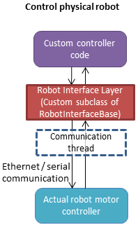
To implement an RIL layer for your robot, you will need to understand details on the communication method used by the manufacturer, e.g., Ethernet, serial, ROS, or some other API. Your RIL implementation should fill out as much of the RobotInterfaceBase methods as provided by the communication layer. The block diagram of the architecture looks like this:

For RIL to work, there are a few functions your subclass will need to fill out, at a minimum:

• numDOFs() or klamptModel()

• Either clock() or controlRate()

• Either setPosition(), moveToPosition(), setVelocity(), setTorque(), or setPID()

• Either sensedPosition() or commandedPosition()

Given these implementations, we provide a convenience class, RobotInterfaceCompleter, that will automatically fill in all other parts of the RIL API, e.g., velocity control, motion queue control, and Cartesian control. (Note: move-to and Cartesian control functions are only available if RobotInterfaceBase.klamptModel is implemented.)

Note

The emulation of some components has rough edges, and this code is subject to change. If you plan to use RIL, we suggest that you install from source so that you can get the latest updates.

Multithreaded Implementations

The best practice for implementing an RIL API is to launch a thread that synchrononously communicates with your robot, while relaying asynchronous commands from the caller. The following code does a very basic job of this for a position-controlled robot, which only relays the sensed/ commanded positions to/from the robot.

from klampt.control.robotinterface import *
from klampt import *
from threading import Thread,Lock

class RobotCommThread:
  def __init__(self,connection):
    Thread.__init__(self)
    self.connection = connection
    self.doStop = False
    self.lock = Lock()
    self.commandedPosition = None
    self.sensedPosition = None
    self.new_commandedPosition = None
    self.status = 'ok'
    self.daemon = True  #flag in Thread that will help kill this Thread under Ctrl+C
  def run(self):
    while not self.doStop:
      with self.lock:
        ...read status, sensedPosition, commandedPosition from the robot...
        ...if disconnected, set status to 'disconnected'...
        if self.new_commandedPosition is not None:
          ...send new_commandedPosition to the robot...
          self.commandedPosition = new_commandedPosition
      #unlock
      time.sleep(0.001) # or some small amount

class MyRIL(RobotInterfaceBase):
  def __init__(self):
    self.thread = None
    self.world = WorldModel()
    self.world.readFile(...path to robot file...)
    self.robot = self.world.robot(0)
  def initialize(self):
    ...connect to the robot, return False if unsuccessful...
    self.thread = RobotCommThread(robot_connection)
    self.thread.start()
  def stop(self):
    if self.thread is not None:
      self.thread.doStop = True
      self.thread.join()
      self.thread = True
  def klamptModel(self):
    return self.robot
  def controlRate(self):
    return ...whatever the robot's control rate is...
  def status(self):
    return self.thread.status
  def commandedPosition(self):
    with self.thread.lock:
      res = self.thread.commandedPosition
    return res
  def sensedPosition(self):
    with self.thread.lock:
      res = self.thread.sensedPosition
    return res
  def setPosition(self,q):
    with self.thread.lock:
      self.thread.new_commandedPosition = q

(Note: a complete implementation will do a better job of error handling.)

ROS Implementations

For a ROS implementation, ROS messaging will already be running in a separate thread, so you don’t need to set up a new thread after you’ve run rospy.init_node(...). This could happen, for example, in the initialize method. Then, for all robot commands provided by your robot’s ROS interface:

1. In the appropriate RIL method, translate the Klamp’t command to a ROS message.

2. Publish the message to the appropriate topic, or call the appropriate service.

For all sensor messages provided by your robot’s ROS interface:

1. In initialize, set up a subscriber to the sensor message.

2. The callback from that subscriber should just store the sensor message.

3. Overload the appropriate RIL method to translate the ROS message to a Klamp’t object. For standard positions, velocities, and torques, use the sensedPosition(), sensedVelocity(), and sensedTorque() methods.

   For more complex, asynchronous items like laser sensors, cameras, RGB-D sensors, and force/torque sensors, you should use the sensors(), sensorMeasurements(), and sensorUpdateTime() methods. For best interpretability (and compatibility with Klampt’s visualization tools, e.g. RobotInterfacetoVis), you should also make sure the sensor is defined in the robot’s klamptModel() model, and that these measurements match the format of the corresponding Klamp’t sensor.

As an example, consult the implementation of RosRobotInterface. This class sends ROS JointTrajectory commands and receives ROS JointState sensor messages.

Frankenstein Robots

Important

New in 0.8.3 and has barely been tested. Use at your own risk.

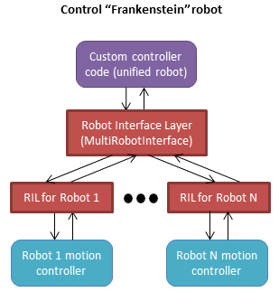
We often build robots out of several components, such as an arm and a gripper, and it can be a pain to coordinate the control of each component. Klamp’t provides a convenience class, MultiRobotInterface, that lets you assemble robots into parts.

Experimental Controller Building Blocks

Important

THESE DOCS ARE OUT OF DATE. The API has changed a lot and the previously meager functionality is only slightly improved in 0.8.3. It is not clear whether this API will be maintained.

A ControllerBlock interface is a very simple object with two important methods:

• advance(self,**inputs): given a set of named inputs, produce a dictionary of named outputs. The semantics of the inputs and outputs are defined by the caller. The block moves forward single time step, performing any necessary changes to internal state.

• signal(self,type,**inputs): sends some asynchronous signal to the controller. The usage is caller dependent.

Optionally, it can also implement inputNames/outputNames, and get/setState.

Robot controller blocks

A ControllerBlock that operates as the top-level controller for a robot is said to follow the RobotControllerBase convention. The input dictionary contains sensor messages, specifically containing the following elements:

• t: the current simulation time

• dt: the controller time step

• q: the robot’s current sensed configuration

• dq: the robot’s current sensed velocity

• The names of each sensors in the simulated robot controller, mapped to a list of its measurements.

The RobotControllerBase output dictionary represents a command message. to be sent to the robot’s low-level motor controllers. A command message can have one of the following combinations of keys, signifying which type of joint control should be used:

• qcmd: use PI control.

• qcmd and dqcmd: use PID control.

• qcmd, dqcmd, and torquecmd: use PID control with feedforward torques.

• dqcmd and tcmd: perform velocity control with the given actuator velocities, executed for time tcmd.

• torquecmd: use torque control.

The klampt_sim script accepts arbitrary feedback controllers in this form. To specify such a controller, provide as input a .py file with a single make(robot) function that returns a subclass of ControllerBlock that implements the desired functionality. For example, to see a controller that interfaces with ROS, see klampt/control/io/roscontroller.py.

Building controllers from blocks

Internally the controller can produce arbitrarily complex behavior. Several common blocks are implemented in klampt.control.blocks.

• TimedControllerSequence: runs a sequence of sub-controllers, switching at predefined times.

• MultiController: runs several sub-controllers in parallel, with the output of one sub-controller cascading into the input of another. For example, a state estimator could produce a better state estimate q for another controller.

• ComposeController: composes several sub-vectors in the input into a single vector in the output. Most often used as the last stage of a MultiController when several parts of the body are controlled with different sub-controllers.

• LinearBlock: outputs a linear function of some number of inputs.

• LambdaBlock: outputs f(arg1,...,argk) for any arbitrary Python function f.

• StateMachine: a base class for a finite state machine controller. The subclass must determine when to transition between sub-controllers.

• TransitionStateMachine: a finite state machine controller with an explicit matrix of transition conditions.

A trajectory tracking controller is given in klampt/control/blocks/trajectory_tracking.py. Its make function accepts a robot model (optionally None) and a linear path file name.

A preliminary velocity-based operational space controller is implemented in control-examples/OperationalSpaceController.py, but its use is highly experimental at the moment.

State estimation

Controllers may or may not perform state estimation.

Using the controller.py interface, state estimators can be implemented as ControllerBlock subclasses that calculate the estimated state objects in the advance() method.