Section II. MODELING
Chapter 7. Representing Geometry
So far we have described methods for reasoning about a robot's spatial reference frames, but have not yet considered the geometric content of those frames, such as the shape and size of the physical structure of each link. Certainly, it would be wise to consider these geometries when developing motions and choosing postures, since a robot should avoid unintentional collision with the environment, and should make contact when desired. Geometry is also important in robot design, since the shape of a robot dictates how well it can squeeze into tight locations, and how much of the surrounding workspace it can reach without self-colliding.
Mathematical and computational representations of geometry have long been studied, and a rich set of techniques are in active use today. They come from a variety of fields, including computer-aided design (CAD), computational geometry, computer graphics, and scientific visualization --- and hence this survey only scratches the surface of the vast variety of geometric representations and calculations.
Example applications
Geometry is used pervasively throughout in robotics, including:
Mechanism design
Physics simulation
Collision avoidance
Proximity detection
Motion planning
Calibration
3D mapping
Object recognition
Visualization and performance evaluation
These applications will require some type of geometric operations to be performed on one or more objects, such as:
Visualization
Collision detection
Distance or closest-point computation
Ray casting
Contact surface computation
Penetration depth computation
Simplification
Shape fitting
Storage and transmission
Due largely to decades of work in high-performance, realistic 3D visualization, many of these operations are extremely fast due to advances in computing hardware (graphics processing units, or GPUs) as well as advanced geometric algorithms and data structures. Nevertheless, it is important for robotics practitioners to understand the performance tradeoffs in choosing representations appropriate for the desired operations.
As an example, consider the problem of computing a collision-free inverse kinematics solution. Assuming we are given 1) an analytical IK solver, 2) geometric models of each robot link, and 3) a geometric model of the environment, this problem can be addressed as follows:
Compute all IK solutions.
For each IK solution, run forward kinematics to determine the robot's link transforms.
Determine whether the robot's link geometries, placed at these transforms, would collide with themselves or the environment.
If any configuration passes the collision detection test, it is a collision-free solution.
Otherwise, no solution exists.
The key step is the collision detection in Step 3. If the models are geometrically complex, collision detection may be a computational bottleneck. But, if they are too simple to faithfully represent the robot's geometry, then the computed solution may either miss a collision (the geometric model is optimistically small) or fail to find valid solutions (the geometric model is conservatively large).
Geometry representations
A geometry $G$ is considered to be some region of space $G \subset \mathbb{R}^2$ or $\mathbb{R}^3$ depending on whether we are considering planar or 3D robots. Geometry representations can be categorized by which part of $G$ is actually represented:
Geometric primitives like points, lines, spheres, and triangles represent a shape $G$ in terms of a fixed number of parameters.
Surface representations approximate only the boundary of $G$, denoted $\partial G$.
Volumetric representations approximate the entirety of $G$: interior, boundary, and exterior.
Point-based representations store a sampling of individual points from $\partial G$.
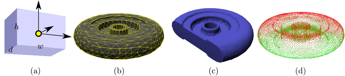
There are a number of tradeoffs involved in choosing representations. In general, surface representations are most widely used for visualization and CAD, while volumetric representations are most useful for representing 3D maps and determining whether points are inside or outside. Point-based representations are widely used to represent raw data from 3D sensors like lidar and depth cameras. Geometric primitives are preferred when speed of geometric operations is prioritized over fidelity.
Geometric primitives
Primitives are the simplest form of geometric representation, and are compact, mathematically convenient, and lend themselves to fast geometric operations: exact calculations can be calculated in constant ($O(1)$) time. (For more information about Big-O notation, consult Appendix C.1.) However, they are the least flexible representation and do not represent most real geometries with high fidelity.
Common primitives include points, line segments, triangles, spheres, cylinders, and boxes. For each primitive type, a primitive's shape is represented by a fixed number of parameters.
A point is specified by its coordinates $(x,y)$ or $(x,y,z)$.
A line segment is specified by the coordinates $\mathbf{a}$, $\mathbf{b}$ of its end points.
A circle (in 2D) or sphere (in 3D) is specified by its center $\mathbf{c}$ and radius $r > 0$.
A triangle is specified by its vertices $\mathbf{a}$, $\mathbf{b}$, $\mathbf{c}$.
A cylinder is specified by its base $\mathbf{b}$, primary axis $\mathbf{a}$, height $h > 0$, and radius $r > 0$.
A box is represented by a coordinate frame $T$ with origin at its corner and axes aligned to the box's edges, and its dimensions on each axis, width/height $(w,h)$ in 2D and width/height/depth $(w,h,d)$ in 3D.
An axis-aligned box with lower coordinate $\mathbf{l}$ and upper coordinate $\mathbf{u}$ contains all points $\mathbf{x} = (x_1,x_2,x_3)$ such that $x_i \in [l_i,u_i]$ for $i=1,2,3$.
These representations are not unique, and are chosen by convention. For example, the origin of a box may be chosen to be its center point rather than a corner.
Surface representations
Surface representations (also known as boundary representations, or b-reps) store the boundary of a geometry $\partial G$ without explicitly representing its interior / exterior.
By far, the most common 3D surface representation is a triangle mesh: a collection of triangles $(\mathbf{a}_1,\mathbf{b}_1,\mathbf{c}_1),\ldots,(\mathbf{a}_N,\mathbf{b}_N,\mathbf{c}_N)$ that mesh together to approximate the geometry's surface. Triangle meshes have two major advantages over other representations: 1) with a sufficient number of triangles, they can approximate arbitrary surfaces, and 2) graphics hardware is highly optimized for visualization of large triangle meshes (as of writing, top-end commodity graphics cards can render over a billion triangles per second). The 2D equivalent is a polygonal chain.
It is important to note that in order to represent a solid surface, the edges of neighboring triangles in the mesh should be coincident, so that most vertices will be represented in several triangles. To save on storage space / representational complexity, triangle meshes are often represented as a vertex list $\mathbf{v}_1,\ldots,\mathbf{v}_M$ and a triangle index list $(i_{a1},i_{b1},i_{c1}),\ldots,(i_{aN},i_{bN},i_{cN})$, where the index triple $(i_{ak},i_{bk},i_{ck})$ indicates that the $k$'th triangle is composed of vertices $\mathbf{v}_{i_{ak}},\mathbf{v}_{i_{bk}},\mathbf{v}_{i_{ck}}$. For example, the cube in Fig. 2 represents a solid, but only the vertices and triangles of the surface are represented.
# Code for the triangle mesh visualization↔
The visualization below loads a triangle mesh from disk, and visualizes it using WebGL. Try spinning it by dragging on it with the left mouse button, and translating it by dragging with the right mouse button.
#Load a chair mesh from disk and visualize it↔
Other common surface representations include:
Convex polygons (in 2D) / Convex polytopes (in 3D): represented by a list of connected faces, edges, and vertices. Also has a volumetric representation in terms of halfplanes $(\mathbf{a}_i,b_i)$, $i=1,\ldots,N$ such that the geometry is determined by the set $G = \{ \mathbf{x} \quad |\quad \mathbf{a}_i \cdot \mathbf{x} \leq b_i, i=1,\ldots,N \}$.
Parametric curves (in 2D) / Parametric surfaces (in 3D): In the 2D case, a function $f(u) : D \rightarrow \mathbb{R}^2$ sweeps out a curve as the parameter varies over a domain $D \subseteq \mathbb{R}$. In 3D, a function $f(u,v): D \rightarrow \mathbb{R}^3$ sweeps out the surface as the parameters vary over a domain $D \subseteq \mathbb{R}^2$.
Subdivision surfaces: Defines the surface as a limit of smoothing / refinement operations on a polygonal mesh. Used primarily in computer graphics.
An important caveat of surface representations is that they may fail to properly enclose a volume. For example, a triangle floating in space is a valid triangle mesh, and two intersecting triangles is also a valid triangle mesh, but neither represents a surface of any enclosed volume. A triangle mesh that does truly bound a volume is known as watertight. Non-watertight meshes are also known as polygon soup.
Volumetric representations
Volumetric representations have the main advantage of being able to perform inside / outside tests quickly, and to be able to quickly modify 2D / 3D maps with new information. All of these items store some function $f$ over a ($d=2$ or 3)-D space that indicates whether a point is inside or outside the geometry.
The function values can be interpreted in several ways, including:
Occupancy map: a binary function $f : \mathbb{R}^d \rightarrow \{0,1\}$ where 0 indicates empty space, and 1 indicates occupied space.
Probabilistic occupancy map: a function $f : \mathbb{R}^d \rightarrow [0,1]$ where 0 indicates certain empty space, 1 indicates certain occupied space, and intermediate values reflect the level of certainty that the space is occupied.
Implicit surface: a function $f : \mathbb{R}^d \rightarrow \mathbb{R}$, defined such that $f(\mathbf{x}) < 0$ denotes the interior of the object, $f(\mathbf{x}) = 0$ is the surface, and $f(\mathbf{x}) > 0$ is the exterior.
Signed distance field (SDF): an implicit surface where $f$ denotes the Euclidean distance to the surface if outside of the geometry, or the negative penetration depth if inside the geometry.
Truncated signed distance field (TSDF): A common variant in 3D mapping, which accepts a truncation distance $\tau$. The values of the SDF with absolute value $> \tau$ are truncated.
Attenuation / reflectance map: a function $f : \mathbb{R}^d \rightarrow [0,1]$ indicates how much a point in space interferes with light, sound, or other signal.
Height field / topograpic map: Sort of a cross between a surface and volume representation, height fields store a 2D function $f(x,y)$ that indicates the height of the surface at the point $(x,y)$. This defines a 3D volume over $(x,y,z)$ such that $z > f(x,y)$ indicates empty space, $z=f(x,y)$ indicates the surface, and $z < f(x,y)$ indicates the interior. Frequently used by mobile robots to represent terrain.
The computational representation of the function itself can also vary, including but not limited to:
Combination of basis functions: $f(x)$ is a linear combination of basis functions $f(x) = \sum_i^m c_i b_i(x)$, where $b_i$ are the (fixed) basis functions. Evaluation is $O(m)$ complexity.
Dense pixel / voxel grid: $f$ is stored a 2D or 3D grid, and evaluating $f(x)$ performs a table lookup. For implicit surfaces, $f(x)$ is typically evaluated using bilinear / trilinear interpolation of the values at the grid vertices. Evaluation is $O(1)$.
Hierarchical grid (quadtree / octree): a hierarchical 2D grid (quadtree) or 3D grid (octree)that stores the function at progressively finer levels, up to a given resolution. Evaluation is $O(\log n)$, with $n$ the number of divisions on each axis.
Sparse grid / hash grid: Stores only important cells or blocks of volumetric data, e.g., the occupied cells of an occupancy map, or non-truncated cells of a TSDF. Evaluation is $O(1)$.
Some 2D examples are illustrated in Fig. 3.

Various combinations of value types and representations are useful for certain tasks. Popular representations include:
- Occupancy grids (occupancy map on a dense voxel grid) are used in the popular video game Minecraft to store a map of a 3D world that can be modified in unlimited ways.
- Probabilistic occupancy grids (probabilistic occupancy map on a dense pixel grid), used in many 2D simultaneous localization and mapping (SLAM) algorithms.
- Occupancy map on an octree, used in the popular OctoMap 3D mapping algorithm.
- TSDF on dense grids, used in small-scale (object or single room) 3D mapping algorithms.
- TSDF on sparse grids, used in large-scale (building-scale) 3D mapping algorithms.
- Attenuation / reflectance grids are used in volumetric medical imaging, like ultrasound, CT, and MRI scans, as well as sonar used in underwater and surface vehicles.
All grid-based representations are defined over a volume, usually an axis-aligned bounding box with corners $\mathbf{l}$, $\mathbf{u}$. The grid will have size $m \times n \times p$, and converting between world space and grid space requires a shift and a scale. In particular, the cell indices $(i,j,k)$ of a point $(x_1,x_2,x_3)$ are determined by a transform \begin{equation} \begin{split} i &= \lfloor m (x_1 - l_1) / (u_1 - l_1) \rfloor \\ j &= \lfloor n (x_2 - l_2) / (u_2 - l_2) \rfloor \\ k &= \lfloor p (x_3 - l_3) / (u_3 - l_3) \rfloor \end{split} \label{eq:PointToGridIndices} \end{equation} where $\lfloor \cdot \rfloor$ is the floor operation that returns the largest integer less than or equal to its argument. (Here we assume zero-based indices.)
Point-based representations
Point-based representations are widely used in robotics to represent environment geometries because they are the type of data directly produced by depth sensors. These representations store a sampling of points $\mathbf{p}_1,\ldots,\mathbf{p}_N$ from the geometry surface $\partial G$. Individual points may be associated with colors, normals, and other information. Usually, this sampling is highly incomplete, exhibiting irregular density or large gaps caused by occlusion.
There are two major types of point-based representations: point clouds and depth images (aka range images). A point cloud is simply an unstructured list of points with no assumption of regularity. Points are not a priori identified to objects, nor to each other. This type of representation results from moving lidar sensors and naively merged depth scans.
A depth image is a 2D grayscale image indicating the distance from the camera sensor to the surface observed by each pixel. (Some invalid dpeth value, such as 0 or $\infty$, indicates no data is available at that pixel). This is the raw form of data returned from depth cameras (Fig. 4). The advantage of this form of representation over point clouds is that nearness in the image implies some notion of spatial proximity in 3D space; furthermore, the line between the camera's focal point and the read point must be free of other geometry. Algorithms can exploit this knowledge for faster geometric operations, which we shall see when we return to the topic of 3D mapping. Knowledge about the camera's position and orientation in space is required to correlate the 2D image to 3D points in a global reference frame.
#Code for showing an RGB-D sensor's color and depth image (axis units in pixels, depth units in m)↔
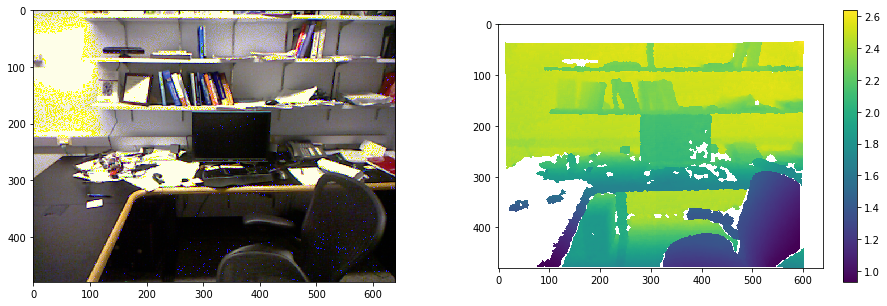
Both point clouds and depth images will be, in general, imperfect representations of geometry due to sensor noise, occlusion, and limited field-of-view.
Accuracy tradeoffs
Except for geometric primitives, each representation can represent geometry at various levels of resolution, such as the density of triangles in a triangle mesh, or the size of voxel cells in an occupancy grid. The choice of representation and its resolution should be chosen to balance several competing demands:
Fidelity to the true geometry
Appropriateness to desired geometric operations
Computational complexity of geometric operations
Difficulty of acquisition / creation
Implementation complexity
Storage and transmission speed requirements
We will discuss several of these aspects below. In terms of fidelity, however, we can see some general trends. First, 3D surface representations (e.g., triangle meshes, point clouds) typically need $O(1/h^2)$ elements to achieve an approximation error of $h$ to a given surface. Volumetric representations based on a 3D grid will require $O(1/h^3)$ grid cells, which can be a substantial burden: consider dividing a 5 m $\times$ 5 m $\times$ 5 m room into centimeter-sized cells: $500\times 500 \times 500 = 125$ million cells would be needed! On the other hand, assuming the surface area of the object is approximately 5 m $\times$ 5 m, a surface-based representation would only need about 25,000 elements to represent the same object.
The use of more advanced data structures like octrees can compress the space complexity of volumetric representation to nearly $O(1/h^2)$, but at the expense of increased complexity of implementing geometric operations.
Representing rigid poses and movement
Because it is so common to represent objects as rigid bodies, it is much easier to model the movement of an object as the movement of an rigid body frame, rather than to explicitly modify the geometry itself. This implicit transformation approach is used ubiquitously in robotics, visualization, and computer graphics. Specifically, we imagine the object to have a local reference frame, and define a local geometry $G_L \subset R^3$ in the local coordinates. The object's pose is a transformation $T$ from the reference frame to the world frame. As the object moves, $T$ changes, but the local geometry data remains static.
Hence, we can represent the set of points contained by the object $G(t) \subset R^3$ at time $t$ given only the pose $T(t)$. The two representations are:
Explicit transformation: $G(t) = \{ T(t)x \quad|\quad x \in G_L \}$. (Imagine the points of the local geometry moving with the object's transform.)
Implicit transformation: $G(t) = \{ x \in R^3 \quad|\quad T(t)^{-1} x \in G_L \}$. (Imagine the points in world coordinates being projected back into the reference frame.)
Because it is much more efficient to change transforms than geometry data, the implicit transformation approach is preferred in most cases, except perhaps geometric primitives. For example, if a triangle mesh with 1,000,000 points undergoes a rotation and translation, this can be calculated using 1,000,000 3x3 matrix-vector multiplies and the same number of 3-vector additions. But, in the implicit representation, we can update a transform only by 1 4x4 matrix multiply (using homogeneous coordinates), or 1 3x3 matrix-matrix multiply, a matrix-vector multiply, and a 3-vector addition (using rotation matrix and translation vectors). Henceforth, we will describe a geometry $G$ in the implicit form as a local-geometry / transform pair $G=(G_L,T)$.
Proximity queries
Proximity queries are an important class of geometric operations for collision avoidance, motion planning, and state estimation. There are many types of queries, with the following being the most typical in robotics:
- Inside-outside (containment) tests: Return a boolean indicating whether a point $\mathbf{x}$ is contained within a geometry $G$.
- Collision detection: Return a boolean indicating whether geometries $A$ and $B$ overlap.
- Distance queries / Closest points: Return the distance between geometries $A$ and $B$, or 0 if they overlap. Usually this requires determining the closest points on each geometry.
- Tolerance queries: Return a boolean indicating whether geometries $A$ and $B$ are within some distance tolerance $\tau$. If the objects are well-separated, this is usually faster than a true distance query.
- Penetration depth queries: If $A$ and $B$ overlap, return the distance by which one must translate to remove the overlap.
- Ray casting: Return a boolean indicating whether a ray $\overrightarrow{ab}$ hits geometry $G$. This query may also return the distance $d$ between $a$ and the first-hit point. Used in user interfaces, e.g., to select objects of interest, rendering, and visibility determination.
- Overlap region estimation: If $A$ and $B$ overlap, return a representation of the area or volume of overlap. Used mainly in physics simulation, manipulation, and legged locomotion.
In this book, we describe inside-outside tests and collision detection in more detail for a small number of geometry representations.
Inside-outside (containment) tests
Inside-outside testing is a straightforward operation for primitives and volumetric representations, but not as straightforward for surface representations. Note that for a implicitly transformed geometry $G=(G_L,T)$, this becomes a problem of determining whether the local coordinates of the point are within the local geometry: $T^{-1}\mathbf{x} \in G_L$.
Geometric primitive containment testing
For primitives like spheres, containment can be tested directly from the mathematical expression of the primitive. For example, a ball with center $\mathbf{c}$ and radius $r$ is defined by: \begin{equation} \| \mathbf{x} - \mathbf{c} \| \leq r. \label{eq:SphereContainment} \end{equation}
An oriented box with coordinate frame $T$ and dimensions $w \times h \times d$ contains all points whose local coordinates lie in the axis-aligned box $[0,w] \times [0,h] \times [0,d]$; hence the test for whether a world-space point lies inside is simply the test: $$T^{-1} \mathbf{x} \in [0,w] \times [0,h] \times [0,d].$$
Volumetric containment testing
Volumetric representations also lend themselves to fast containment testing. Implicit surfaces, including SDFs and TSDFs, simply require evaluating the sign of $f(\mathbf{x})$. Grids have O(1) containment testing by converting the point to grid coordinates using Eq. $(\ref{eq:PointToGridIndices})$ and then retrieving the contents of the identified grid cell. Octrees containment testing is typically logarithmic in the number of grid cells.
Surface containment testing
Surface representations are more challenging since there is no explicit representation of the object's interior. If it is known that a surface representation is watertight, then it is possible to count the number of intersections between the surface and a ray whose origin is $\mathbf{x}$ and direction is arbitrary. If the number of intersections is odd, then the point is inside; otherwise it is outside.

There is, however, some subtlety when the ray lies directly tangential to the surface and/or passes through an edge of the mesh (Fig. 5, right). These must be handled when developing a robust algorithm.
Collision detection between primitives
Collisions between geometric primitives can be computed through closed-form O(1) expressions. We shall give a couple of useful definitions here.
Sphere vs sphere. Two spheres with centers $\mathbf{c}_1$ and $\mathbf{c}_2$ and respective radii $r_1$ and $r_2$ overlap when the distance between the two centers is no larger than the sum of the radii: $$\| \mathbf{c}_1 - \mathbf{c}_2 \| \leq r_1 + r_2.$$
Sphere vs line. A sphere overlaps an infinite line iff the closest point on the line to the sphere's center falls inside the sphere. Suppose the sphere has center $\mathbf{c}$ and radius $r$, and the line is given by two points on the line $\mathbf{a}$ and $\mathbf{b}$. Then, the closest point $\mathbf{p}$ to the center is determined through projection of $\mathbf{c}$ onto the line: \begin{equation} \mathbf{p} = \mathbf{a} + (\mathbf{b} - \mathbf{a})\frac{(\mathbf{c} - \mathbf{a}) \cdot (\mathbf{b} - \mathbf{a})}{\| \mathbf{b} - \mathbf{a} \|^2}. \end{equation} Then, containment of $\mathbf{p}$ is determined through ($\ref{eq:SphereContainment}$).
Sphere vs line segment. Similar to the sphere vs line case, but we must handle the case in which the closest point from $\mathbf{c}$ to the line defining the segment falls outside of the endpoints. Let the line segment be defined by endpoints $\mathbf{a}$ and $\mathbf{b}$. Notice that the scalar parameter determined by projection $$u = \frac{(\mathbf{c} - \mathbf{a}) \cdot (\mathbf{b} - \mathbf{a})}{\| \mathbf{b} - \mathbf{a} \|^2}$$ defines what fraction $\mathbf{p}$ interpolates between $\mathbf{a}$ and $\mathbf{b}$. To restrain $\mathbf{p}$ to the line segment, we can limit $u$ to the range $[0,1]$. In other words, we compute whether the sphere contains the point: $$\mathbf{p} = \mathbf{a} + (\mathbf{b} - \mathbf{a})\max\left(0,\min \left(1,\frac{(\mathbf{c} - \mathbf{a}) \cdot (\mathbf{b} - \mathbf{a})}{\| \mathbf{b} - \mathbf{a} \|^2}\right)\right).$$
Line segment vs line segment (2D). For two 2D line segments, defined respectively by endpoints $\mathbf{a}_1$ and $\mathbf{b}_1$ and endpoints $\mathbf{a}_2$ and $\mathbf{b}_2$, the collision point can be determined as follows. First, determine the intersection point of the two supporting lines by solving two simultaneous equations: $$\mathbf{a}_1 + u (\mathbf{b}_1 - \mathbf{a}_1) = \mathbf{a}_2 + v (\mathbf{b}_2 - \mathbf{a}_2)$$ where $u$ gives the interpolation parameter of the first line, and $v$ gives the interpolation parameter of the second line. The solution $(u,v)$ can be determined through $2\times 2$ matrix inversion: $$\begin{bmatrix}{b_{1,x} - a_{1,x}} & {a_{2,x} - b_{2,x}} \\ {b_{1,y} - a_{1,y}} & {a_{2,y} - b_{2,y}} \end{bmatrix}\begin{bmatrix} u \\ v \end{bmatrix} = \begin{bmatrix}{a_{1,x}-a_{2,x}} \\ {a_{1,y}-a_{2,y}} \end{bmatrix}$$ If a solution $(u,v) \in [0,1]^2$ exists, then the two line segments collide. (In 3D, two line segments are unlikely to collide, so this overdetermined system is unlikely to have a solution.)
AABB vs AABB. Two axis-aligned bounding boxes overlap if all of the individual axis-wise intervals overlap. Two intervals $[a,b]$ and $[c,d]$ overlap if $a \in [c,d]$, $b \in [c,d]$, $c \in [a,b]$, or $d \in [a,b]$.

Separation principle for convex objects
It is somewhat more challenging to determine whether triangles intersect each other, or two non-aligned boxes intersect each other. However, we can use a general separation principle that holds between all convex objects. The principle, illustrated in Fig. 5, is as follows:
If $A$ and $B$ are convex objects, $A$ and $B$ overlap if and only if there does not exists a plane separating them.
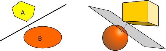
We can use this fact as follows. Let $\mathbf{n}$ be some direction in space. Suppose $\mathbf{n} \cdot \mathbf{x}$ over all $\mathbf{x} \in A$ spans the range $[a,b]$, and $\mathbf{n} \cdot \mathbf{x}$ over all $\mathbf{x} \in B$ spans the range $[c,d]$. If the projected intervals $[a,b]$ and $[c,d]$ do not intersect, then we can definitively say that $A$ and $B$ do not intersect.
It is straightforward to determine these intervals for a convex polygon with vertices $\mathbf{v}_1,\ldots,\mathbf{v}_n$. The projected distances along $\mathbf{n}$ are $\mathbf{n} \cdot \mathbf{v}_1, \ldots, \mathbf{n} \cdot \mathbf{v}_n$, and we can simply take the minimum and maximum to determine the projected interval $[\min_{i=1}^n \mathbf{n} \cdot \mathbf{v}_i, \max_{i=1}^n \mathbf{n} \cdot \mathbf{v}_i]$.
The question is now how to determine which directions $\mathbf{n}$ to use. For many shapes we can define a finite number of directions $\mathbf{n}_1,\ldots,\mathbf{n}_k$ such that failure to find a separation along all directions proves that a the geometries do not overlap. Examples are as follows.
Collision detection between convex polygons in 2D
Suppose convex polygons $A$ and $B$ are respectively given by points $\mathbf{a}_1,\ldots,\mathbf{a}_m$ and $\mathbf{b}_1,\ldots,\mathbf{b}_n$, listed in counter-clockwise order. Then, the $i$'th edge of $A$ has an outward normal direction $$\begin{bmatrix}{a_{i,y} - a_{(i\mod m)+1,y}} \\ {a_{(i\mod m)+1,x} - a_{i,x}} \end{bmatrix}$$ and the $j$'th edge of $B$ has an outward normal direction $$\begin{bmatrix}{b_{j,y} - b_{(j\mod n)+1,y}} \\ {b_{(j\mod n)+1,x} - b_{j,x}} \end{bmatrix}$$ where the modulo is needed to ensure proper wrapping around when $i=m$ or $j=n$. Applying the separation principle to all such normal directions gives a straightforward way to determine whether the polygons overlap.
Another approach, which generalizes to non-convex polygons, is to calculate segment-segment intersection between each pair of edges along the polygon. This test fails, however, when one polygon is contained within another. Hence, to be certain that a polygon does not overlap the interior of another, we can follow the test by determining whether any point of A lies within B, and vice versa.
Collision detection detween convex polytopes in 3D
3D convex polytopes consist of vertices, edges, and faces. Each edge is bordered by two vertices and two faces, and each face is bordered by some number of edges and an equal number of vertices. The approach of examining for separation along each face of each object runs the risk of failing to determine separation in certain cases. The problem is that in 3D, the two closest features on the polytope could be two edges, rather than a point to a face. Hence we must augment the number of directions examined for separation to handle this case. Specifically, for each combination of edges $(\mathbf{a}_1,\mathbf{a}_2)$ on $A$ and $(\mathbf{b}_1,\mathbf{b}_2)$ on $B$ we should determine whether separation holds along the direction: $$(\mathbf{a}_2 - \mathbf{a}_1) \times (\mathbf{b}_2 - \mathbf{b}_1).$$ If separation does not hold with respect to each normal direction of each face and each cross product direction, then the two polytopes overlap.
Although this algorithm may be straightforward, it may be quite inefficient for complex polytopes. A substantially more efficient method is known as the GJK algorithm. This algorithm maintains a point in each geometry, $\mathbf{x}_A \in A$ and $\mathbf{x}_B \in B$, as well as which boundaries are met at the point (Fig. 8). It proceeds by iteratively "walking" the points toward one another to reduce the distance between them. Each step for a point is as follows (the steps for $\mathbf{x}_A$ are shown, they are symmetric for $\mathbf{x}_B$):
If $\mathbf{x}_A = \mathbf{x}_B$, the polytopes overlap and we are done.
Determine the set of faces $F = \{f_1,\ldots,f_k\}$ met at $\mathbf{x}_A$. If the dot product between the direction $\mathbf{x}_B - \mathbf{x}_A$ and the normal of a face is negative, remove it from $F$.
If $|F| = 0$, then $\mathbf{x}_A$ is an interior point. Walk straight along the line segment toward $\mathbf{x}_B$ until $\mathbf{x}_A = \mathbf{x}_B$ or a boundary is hit.
If $|F| = 1$, then $\mathbf{x}_A$ is on a face. Project the direction $\mathbf{x}_B - \mathbf{x}_A$ on the plane supporting the face. Walk along this direction until the projected end point is reached, or an edge about the face is hit.
If $|F| = 2$, then $\mathbf{x}_A$ is on an edge. Walk along the edge in the direction $\mathbf{x}_B - \mathbf{x}_A$ projected onto the edge. Walk along this direction until the endpoint is reached, or a vertex is hit.
If $|F| \geq 3$, then $\mathbf{x}_A$ is on a vertex. It remains at the vertex.
If at two subsequent iterations both $\mathbf{x}_A$ and $\mathbf{x}_B$ fail to move, then $\mathbf{x}_A$ and $\mathbf{x}_B$ are closest points, and the algorithm is done.

Although $A$ and $B$ may have $m$ and $n$ faces, respectively, polytopes usually have a constant number of edges per face and faces per vertex. Because we can track which faces are met at each point, the most expensive operation in this algorithm is the interior $|F|=0$ case, where each plane must be checked for intersection with the line segment $(\mathbf{x}_A,\mathbf{x}_B)$. However, we can show that this operation occurs at most once. Assuming we can perform the bookkeeping to keep track of which edge borders which face, which faces border which vertex, etc. each subsequent step takes constant time. As a result, the entire algorithm takes $O(m+n)$.
For some tasks, such as physics simulation, we can do even better by exploiting temporal coherence in the movement of each polytope. Observe that if $A$ or $B$ move just a little bit, the closest points are likely to be on the same features or on nearby features. Hence, by keeping track of the closest points and features over time, each update can be quite fast. In practice, updates are typically $O(1)$.
Bounding volume hierarchies
For more complex, non-convex representations like triangle meshes, the approach of checking each pair of primitives defining the objects is prohibitively expensive. Instead, hierarchical geometric data structures known as bounding volume hierarchies (BVHs) are used to accelerate collision detection as well as other geometric operations. The approach consists of two general ideas.
First, portions of a geometry can be bounded by simple primitive bounding volumes (BVs), which provides a quick-reject test to eliminate more expensive computations. Suppose it is known that geometry $A$ lies entirely within a sphere $S_A$ and $B$ lies within a sphere $S_B$. Then, if $S_A$ and $S_B$ do not overlap, it is certain that $A$ and $B$ do not overlap. Spheres and (oriented) boxes are commonly used as primitive BVs.
Second, a "divide and conquer" approach can be used where if two top-level BVs overlap, we can divide the two model into portions that are themselves contained within smaller BVs. This division is performed recursively, leading to smaller and smaller portions of the model until individual primitives are left. The BVH stores all of these BVs in a hierarchical data structure (a tree) with the top level bounding volume (the root) containing the entire model, and the lowest level (the leaves) containing individual primitives. The BVH is precomputed for a given model and then reused during collision detection.

BVH representation and computation
A BVH is a hierarchical data structure $H$ defined with respect to the local frame of each geometry (recall the implicit representation $G=(G_L,T)$). The contents of a leaf node $N$ are a portion of $G_L$, such as the lowest-level primitives of a triangle mesh or point cloud. A non-leaf node $N$ is associated with a subset geometry $G_L(N)\subseteq G_L$ contained in the leaves of the subtree of $N$. $N$ stores a bounding volume $B(N)$, which is a geometric primitive (defined in the local frame) that is guaranteed to contain all of $G_L(N)$. The children of $N$ contain smaller subsets of $G_L(N)$, while for the root node $G_L(N)=G_L$.
Note that if the geometry moves according to a rigid transform, the precomputed BVH still applies to the local geometry, with the implicit understanding that any collision computations will take place in the world frame. In other words, we delay transforming any primitives and bounding volumes to the world frame until just before each geometric operation takes place.
The BVH structure is an important determinant of ultimate collision query performance. For best performance, we would like the BVH to satisfy several properties:
- Balanced. The BVH should be a balanced tree to minimize its height.
- Tightness. The BVs of non-leaf nodes $N$ to be tightly wrapped around the geometry $G_L(N)$ contained therein, so that portions of the geometry can be pruned quickly.
- Spatial coherence. Child BVs should contain portions of the geometry that are separated as far as possible to encourage fast pruning. (This is related to tightness.)
A BVH is typically created either in top-down or bottom-up fashion. Top-down construction uses a recursion on a subset $S \subseteq G_L$, which is initially set to $S=G_L$ itself. If $S$ is small enough (contains one or a few primitives), then a leaf node $N$ is output with $S$ as its contents. Otherwise, the BV for $S$ is constructed, a non-leaf node $N$ is instantiated, and the children are $N$ are recursively constructed by subdividing $S$ into two (or more) parts. To encourage tightness and spatial coherence, one approach is construct the subdivision by finding a dividing plane, and create two children containing primitives on either side of the plane. To encourage balance, the dividing plane should approximately divide $S$ into two subsets of equal size.
In bottom-up fashion, a leaf node is constructed for each primitive. Then, pairs of nearby or highly overlapping nodes are aggregated into non-leaf nodes. This process repeats until only one node remains (the root). There is a choice here about how to construct a BV of two aggregated nodes. Either the BV could be constructed by bounding the children BVs (looser but faster), or by bounding the underlying geometry (tighter but slower).
Both processes are relatively expensive, with top-down computation taking at least $O(n h)$ time, where $h$ is the height of the BVH tree, and bottom-up computation taking at least $O(n \log n)$ time, depending on how efficiently pairwise aggregation can be performed. However, the expense is worthwhile particularly if it can be amortized over many collision queries.
If the geometry $G_L$ itself changes frequently, then the BVH must be recomputed. If the change is slight, then the same tree structure can be reused with only minor changes to the BVs. For example, for non-rigid deformations, the BVs can be recomputed in bottom-up fashion to reflect the new geometry after transformation. However, if the change is drastic, then the BVH should be computed from scratch. For example, if a straight rope gets tied into a bow, then an optimal BVH for the bow would group together the parts of the rope that are knotted.
BVH queries
To check collision between two BVHs $H_A$ and $H_B$, the following operations are performed recursively, starting at the root BVs.
If the two BVs do not overlap, return "no collision".
If the two BVs are leaves, test their contents for collision. If a collision exists, return "collision".
Otherwise, pick one of the BVs and recurse on both of its children. If either call returns "collision", then return "collision".
(Note: each collision query is performed in world space by transforming the local BVs to world coordinates.)
In step 3, a simple heuristic is to choose the larger of the two BVs. Furthermore, we should choose which child to recurse on first in order to find a collision faster, if one exists. (If the objects collide, recursing on the correct child first may eliminate unnecessary computation with the second child; if they don't collide, both children will need to be checked anyway.) One such heuristic is to start with the child with the greatest volume of overlap with the un-split BV.
Other proximity queries, like distance queries and ray casting, can also be greatly accelerated by BVHs. These are left as exercises for the reader.
Performance
The BVH approach has been extremely successful in practice, and is implemented in several widely used collision detection packages, such as PQP and FCL. Computational performance is generally quite good: on modern PCs, millions of collision checks can be performed per second between meshes consisting of thousands of triangles.
However, the computation cost does vary with the spatial proximity of the objects. If the objects are far from each other, the algorithm is quite fast because only the top level BVs will be checked. If the objects are highly overlapping, then the heuristic will likely lead the search to find a collision quickly, and typically takes logarithmic time. The most expensive case is when the objects have many primitives that are very close to colliding, but not quite.
Broad phase collision detection
The above discussions applied only to pairs of geometries. If $n$ objects are moving simultaneously, then it may be quite expensive to check all $n(n-1)/2$ pairs ($O(n^2)$ time). The process of eliminating pairs of objects from consideration, before performing more detailed collision checking, is known as broad phase collision detection and can lead to major performance improvements when $n$ is large.
One simple method for broad phase collision detection is a spatial grid method, and is most applicable for objects of relatively similar size. Assume that all objects have diameter $d$, and relatively few objects overlap. Then, we can construct a grid where each cell has dimensions $d \times d \times d$, and each cell contains a list of objects whose center lies inside it. This grid can be constructed in $O(n)$ time, particularly when using a sparse data structure like a hash table.
Then, to query for collisions, we loop through all grid cells, and only check collision between objects contained in a cell and each neighboring cell (for a total of 9 cells in 2D and 27 cells in 3D). If the number of objects whose center lies in a grid cell is bounded by a constant, then all pairs of potentially colliding objects can be determined in $O(n)$ time.
This basic scheme can be extended to objects of varying size, or varying query sizes. For example, Fig. 10 shows an application to crowd simulation, in which each agent only needs to consider interacting with agents within some "proximity radius".

Visualization
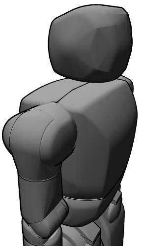
It is important to be able to visualize geometric models, and the chosen representation does effect the performance, realism, and clarity of a visualization. Note that some systems may represent objects' visualization geometries separately from the geometries used for collision detection to make collision detection queries faster; this is typical in the URDF files used in ROS (Fig. 11).
| (a) High-resolution visualization geometry | (b) Lower-resolution collision geometry |
|---|---|
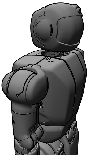 |
 |
Rasterization
The basic operation performed by commodity graphics cards is known as rasterization, in which triangles are drawn, pixel by pixel, into the image shown on a computer screen. The most common frameworks for doing so are the OpenGL (multi-platform) and DirectX (Windows) APIs.
For optimal performance, static or rigidly transforming triangle meshes should be uploaded (once) to the computer's graphics processing unit (GPU). Doing so, modern GPUs can render scenes composed of tens of millions of triangles per frame at real-time rates. Deforming triangle meshes require data to be transferred to the GPU whenever they change, which incurs a performance penalty.
To use rasterization methods to render non-triangle mesh data, the geometry representation must be converted to triangle mesh form. Methods for doing so will be discussed in Section 5.
Colors, lighting, textures, shadowing, and other visual effects may be applied as well to obtain more realistic-looking results. Colors and lighting can be computed on GPUs with relatively straightforward calculations. However, more sophisticated effects like transparency and shadowing require carefully designed rasterization pipelines. Graphics engines such as Unity, Unreal Engine, Blender, Ogre3D, and Three.js provide such functionality in a relatively easy-to-enable manner. But designing such pipelines from scratch, e.g., using OpenGL or DirectX, is an advanced subject studied in computer graphics, and is beyond the scope of this book.
Volumetric rendering
The most common method for visualizing volumetric geometries is to convert the volume to a surface representation and use rasterization techniques. However, it is worth mentioning some other methods for visualizing volumetric data developed for scientific visualization and computer graphics.
Ray-casting methods imagine a ray emanating from each pixel in the screen, and march along through space until a surface is hit. The method is used in computer graphics to render shadows and transparency, as well as for volumetric rendering. Complex visual phenomena like absorption, scattering, and self-shadowing can be simulated using these techniques.
Volumetric texturing methods treat the volume as a 3D texture and rasterize slices through the volume. This approach makes advanced use of modern GPUs to obtain faster frame rates than ray-casting methods.
Point cloud visualization
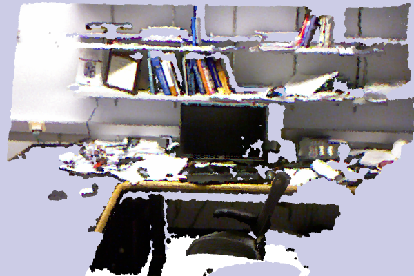
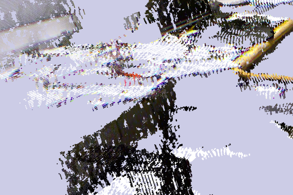
Point clouds can be somewhat challenging to visualize sensibly because the data is distributed with non-uniform sparsity, with missing patches due to occlusion, and spurious noise. If color information is unavailable, simply rasterizing points tends to obscure shape due to the lack of visual cues like lighting. As a result a point cloud, particularly when viewed from oblique angles, will look fairly strange, and will display portions of the objects that should be hidden from view (Fig. 12).
| (a) A point cloud, from a similar vantage point to the camera | (b) A close up of the desk, from another vantage point |
|---|---|
 |
 |
A variety of techniques have been developed to make point cloud visualization more interpretable, such as false color, which encoding $x$, $y$, $z$ position as some sort of color; billboarding which visualizes a small patch of geometry like a square or disk at each point; or splatting, which fills in space between points to make the image appear like a solid object.
Geometric conversions
Given that some geometric operations are more suited to certain representations than others, it is often necessary to perform conversions between representations. It is also often necessary to perform modifications to an existing representation for purposes of computational efficiency, or limitations of storage / transmission channels.
Surface to triangle mesh
Alternate surface representations are often converted to triangle meshes for visualization, collision queries, and compatibility. Parameterized surfaces can be converted to triangle meshes by defining a grid in parameter space, and computing triangles connecting the points on the grid. The resolution of the grid should be chosen carefully to balance computational complexity and geometric fidelity requirements. Subdivision surfaces maintain a polygonal mesh, and by performing recursive subdivision and smoothing operations, the mesh is progressively modified toward a limiting smooth surface. The recursion stops when a desired resolution level is met.
Volume to surface
Implicit surfaces like signed distance functions are typically converted to triangle meshes by the marching cubes algorithm. It operators as follows. First, if the implicit function is not already in grid form, a grid containing the geometry is defined and the surface evaluated on each of the grid points. Then, the algorithm "marches" along each cell, and if the function values of the 8 vertices of the cell contain both positive and negative values, then the 0 isosurface passes through the cell. For cells containing the surface, marching cubes generates anywhere from 1 to 4 triangles within the cell that separate the positive and negative vertices from each other. Repeating this for each cell through the volume produces a watertight isosurface.

Occupancy grids are often converted to triangle meshes by outputting a rectangle when an occupied cell borders an unoccupied one. This has the effect of creating a jagged "stair step" appearance because each face is axis-aligned.
Surface to volume
It is typically harder to convert between surface and volume representations due to subtle resolution issues, and furthermore when a surface is non-watertight it is not even clear what an appropriate volume should be.
From surface to distance field
In the watertight surface case, the fast marching method (FMM) can be used to produce a signed distance field. The first step of FMM is to define a grid containing the surface, and identify all of the surface cells. The signed distance from each grid vertex to the surface is then computed. These seed values are stored in a priority queue, ordered by increasing absolute distance. Additionally, each grid vertex is labeled as either far, considered, or accepted, depending on whether the value at that vertex is not considered yet, tentatively assigned but potentially changing in the future, or fixed.
The seed values are initially marked as accepted. Then, the algorithm proceeds to establish distance values throughout the whole volume in "brush fire" fashion, with the invariant that a vertex is only accepted when all possible direct paths to it from the surface have been considered. The iteration performs the following steps: 1) the grid vertex in the queue with least distance is chosen, and it is marked as accepted, 2) using its distance value, the distance field is extrapolated to its un-accepted neighbors. During step 2, far neighbors are marked as considered, and the distance of a considered vertex is modified only if the extrapolated value is less than the previously stored values. This continues until all vertices are accepted.

Given a suitably defined queue data structure, the overall running time of the algorithm is $O(N \log N)$ where $N$ is the number of grid cells. The major caveat with this algorithm is that the initial determination of inside and outside vertices is sensitive to the grid resolution, and if there are features of the surface smaller than the grid cell size, this may lead to an inconsistent propagation of inside / outside cells.
Implicit surface fitting
Another class of volumetric construction methods attempts to fit an implicit surface function to the surface data. In one common form, an implicit function can be defined as a sum of $N$ radial basis functions : $$f(\mathbf{x}) = \sum_{j=1}^N w_j \phi(\| \mathbf{x} - \mathbf{c}_j \|)$$ where each basis function is defined by the kernel $\phi$ and the center $\mathbf{c}_j$. Here $w_j$ is the weight associated with the $j$'th basis function. Common functions for $\phi$ include the linear kernel $\phi(r) = r$, the Gaussian kernel $\phi(r) = e^{-b r^2}$ with $b$ a constant parameter, and the thin plate spline kernel $\phi(r) = r^2 \log r$.
If we are given $N$ desired function values $f_i$ at points $\mathbf{x}_i$, $i=1,\ldots,N$, then the weights $w_1,\ldots,w_N$ can be tuned so that the function meets those values: $f(\mathbf{x}_j) = f_j$. This fitting is performed by solving a linear system of equations: $$\begin{bmatrix} \phi(\|\mathbf{x}_1 - \mathbf{c}_1 \|) & \cdots & \phi(\|\mathbf{x}_1 - \mathbf{c}_N \|) \\ \cdots & \ddots & \cdots \\ \phi(\|\mathbf{x}_N - \mathbf{c}_1 \|) & \cdots & \phi(\|\mathbf{x}_N - \mathbf{c}_N \|) \end{bmatrix} \begin{bmatrix}{w_1} \\ {\cdots} \\ {w_N} \end{bmatrix} = \begin{bmatrix}{f_1} \\ {\cdots} \\ {f_N} \end{bmatrix}$$
It is then a matter to decide where to place the evaluation points, desired function values, and basis function centers. Certainly, placing points on the geometry surface such that $f(\mathbf{x})=0$ ensures that the implicit surface will pass through these points. However, these points are insufficient, because this leads to the trivial solution $w_1,\ldots,w_N = 0$. An additional constraint is to keep points outside of the geometry to be positive, and some points inside the geometry to be negative. Commonly, these are points offset from the surface along the normal direction. To place the centers, one commonly used technique is to assume the evaluation points and centers shall coincide: $\mathbf{x}_i = \mathbf{c}_i$.
These techniques are susceptible to numerical difficulties when $N$ is large and the evaluation points are close together, since the matrix to be inverted becomes large and ill-conditioned. Running times also suffer with large $N$. More advanced approaches have been developed to overcome these issues, such as using basis functions that lead to a sparse matrix, or fitting many local implicit surfaces over local regions and then combining their results.
Space carving
Space carving techniques will be described in more detail when we discuss 3D mapping, but here we shall give a short overview. The idea is start with a fully occupied occupancy grid, and then to imagine taking views of the surface from multiple angles. For each point in the view, free space is "carved" out of the occupancy grid by marching along a ray emanating from the viewpoints and terminating once the object's surface is reached.
After many views are simulated, the resulting occupancy grid contains the object and matches its silhouette from multiple angles. It is also possible to modify the method slightly to define an approximate signed distance function. It should be noted, however, that space carving methods do not faithfully represent objects with interior cavities or deep holes that are difficult to see from a distant exterior view.
Point cloud to surface
Point clouds can be converted to surfaces in a few ways, but this operation is not trivial because it is not immediately clear simply from the coordinates of a set of points whether they belong to the same surface. As a result, each of these techniques is prone to certain artifacts.
For depth images, it is a simple matter to view the image as a triangle mesh grid and then to assign coordinates to the vertices of the mesh using the depth values and camera transform. Discontinuities in depth can be assumed to be caused by disjoint objects, and triangles corresponding to those discontinuities can be deleted from the mesh.
Another class of techniques first builds a volumetric representation, such as by implicit surface fitting or space carving, and then converts back to a triangle mesh using marching cubes. One such popular technique is known as Poisson reconstruction.
A final class of techniques attempts to build a triangle mesh directly from the point cloud. Some geometric criterion is used to define whether a particular candidate line (in 2D) or triangle (in 3D) connecting points should be included in the surface. Examples of such criteria are $\alpha$-shapes, Delaunay triangulations, and the Voronoi diagram. These methods generally assume that the sampling of points on the surface is sufficiently dense so that, loosely speaking, surface elements are smaller than non-surface elements.
Simplification
Geometry can be simplified in a number of ways for improved computational performance and compact storage / transmission. Point clouds and volumetric representations can be downsampled or averaged to obtain a coarser resolution. Triangle meshes can be simplified in a number of ways. Decimation collapses vertices and/or edges to obtain progressively fewer triangles while attempting to maintain high quality. Clustering methods break the mesh into pieces and then replaces the pieces with simplified re-meshed geometry. A mesh could also be converted into a volumetric representation of a given resolution, and then the surface could be extracted.
Software
There are many software libraries for handling geometric computations, including:
Low-level rasterization: OpenGL (C, with bindings for other languages), DirectX (C++), WebGL (Javascript, based on OpenGL)
Medium-level visualization, scene graph libraries: OpenSceneGraph (C++), OGRE (C++), VTK (C++,Tcl/TK,Python,Javascript), PyInventor (Python), Three.js (Javascript)
High-level game engines: Unity (C#), Unreal Engine (C++)
Collision detection: FCL (C++), Bullet (C++, Python), Shapely (Python, 2D only)
Multifunction: Klamp't (C++, Python) provides visualization and scene-graph functionality, collision detection, and geometric conversion tools.
There are also a plethora of standalone programs for authoring, editing, capturing, and processing geometries.
3D modeling: Blender (free), Sketchup (free), Autodesk Fusion, Solidworks
3D mesh / point cloud editing : Meshlab, VRMesh, CloudCompare
Summary
Key takeaways:
The four main types of geometry representations are primitives, volumes, surfaces, and points.
Each representation has certain strengths and weaknesses with regards to the storage complexity, time complexity, and accuracy of operations that can be calculated upon them.
Collision detection can be performed using mathematical operations for primitive objects, the separation principle for convex objects, or bounding volume decompositions for compound objects.
Conversions between representations is often easiest from volume to surface and from surface to points, while the reverse is much harder.
Exercises
Write pseudocode to fully develop the convex polygon-polygon collision detection algorithm described above. What is the time complexity of this algorithm? Your answer should be in terms of $m$ and $n$, the number of vertices of each polygon.
Write pseudocode to fully develop the polygon-polygon collision detection algorithm for non-convex polygons briefly described above. What is the time complexity of this algorithm? Your answer should be in terms of $m$ and $n$, the number of vertices of each polygon.
Devise pseudocode for determining whether a point cloud intersects with an implicit surface, both of which are represented in implicitly-transformed fashion. (A brute-force method is fine.) Can you generalize this pseudocode to other types of geometry, provided that an inside-outside containment tester is given?
Implement the grid-based broad-phase collision detection technique described in Section 3.5 for disk-shaped objects. Compare the running time of this algorithm with the brute- force collision detection with varying numbers of objects, added at random.
Investigate what geometry representations can be imported and exported from a CAD program (e.g., Solidworks, AutoCAD). Investigate what geometry representations are directly available from an RGB-D camera (e.g., Microsoft Kinect, Intel Realsense). Investigate what geometry representations are used in a 3D mapping program (Google Project Tango, Pix4D, AutoCAD Map 3D).
Suppose that you are implementing a 3D mapping algorithm for mobile indoor robots and wish to map volumes between 5m x 5m x 4m (single room) up to 200m x 200m x 30m (multiple floors of a building). Specify the memory requirements for a 3D grid representation, a triangle mesh representation, and a point cloud representation. Suppose that you store RGB colors in a 32-bit integer, positions (if necessary) as single-precision floating point numbers, and desire a map with spatial resolution of 5cm.
A bounding volume hierarchy can be defined with different types of shapes. Consider the pros and cons of using 1) spheres, 2) axis-aligned bounding boxes, and 3) oriented boxes. Which shape(s) is expected to have the tightest fit to the geometry? Which shape(s) has the fastest bounding volume / bounding volume collision test? Which shape(s) do not need to be explicitly updated when the geometry undergoes a rigid transformation?
Experimentally investigate the running time of bounding volume hierarchy collision detection software. First, examine how precomputation time varies with the complexity of the model. Is the running time linear, quadratic, or something else? Next, examine how query time varies with the complexity of the two models and their proximity. Explain your observations in terms of how many bounding volumes are checked.
Write pseudocode for performing a ray-cast query for a triangle mesh in brute-force fashion. Assume a subroutine is available for computing ray-triangle intersections, called
rayTriangleIntersect(a,b,triangle)whereais the ray start point,bis a point along the ray, and it returns the distancedto the intersection point if there is an intersection, and returnsd=$\infty$ if there is no intersection. Then, write pseudocode for an accelerated version a using a bounding volume hierarchy. Assume a subroutine is available for compute ray-BV intersections, calledrayBVIntersect(a,b,BV).An autonomous vehicle or wheeled mobile robot will sense an environment in 3D, but navigates essentially on a 2D semi-planar ground. Suppose that a laser sensor is used to provide information about the ground surface and obstacles in the form of a 3D point cloud. Suppose the robot knows where it is, and where its sensor is located on its chassis. What processing steps would need to take place to convert the 3D data into a 2D obstacle map assuming that the ground was almost entirely flat (say, with height variation below 2cm)? What would complicate this process if the ground is not flat, such as curbs, hills, speed bumps, and ramps? What information might be available in the point cloud for you to treat curbs as obstacles, but not hills, speed bumps, and ramps? What complications would arise when due to the nature of point cloud data?