Kinematics is the study of the relationship between a robot's joint coordinates and its spatial layout, and is a fundamental and classical topic in robotics. Kinematics can yield very accurate calculations in many problems, such as positioning a gripper at a place in space, designing a mechanism that can move a tool from point A to point B, or predicting whether a robot's motion would collide with obstacles. Kinematics is concerned with only the instantaneous values of the robot's coordinates, and ignores their movement under forces and torques (which will be covered later when we discuss dynamics). The kinematics problem may be rather trivial for certain robots, like mobile robots that are essentially rigid bodies, but requires involved study for other robots with many joints, such as humanoid robots and parallel mechanisms.
This chapter will describe the kinematics of several common robot mechanisms and define the concepts of configuration space and workspace. It will also present the process of forward kinematics, which performs the geometric calculations needed to map configuration space to workspace.
Configuration space and workspace
A robot's kinematic structure is described by a set of links, which for most purposes are considered to be rigid bodies, and joints connecting them and constraining their relative movement, for example, rotational or translational joints.
A robot's layout, at some instant in time, can be described by one of two methods:
A list of coordinates for each joint (typically an angle or translation distance) expressed relative to some reference frame, aka zero position.
A spatial representation of its links in the 2D or 3D world in which it operates, e.g., matrices describing the frame of each link relative to some world coordinate system.
The list of joint coordinates are known as the configuration of the robot. The 2D or 3D world in which the robot lives is known as its workspace.
The importance of a configuration is that it is a non-redundant, minimal representation of the robot's layout. This stands in contrast to the representation of storing each link's frame (also known as maximal coordinates), but the constraints imposed by each joint might not be satisfied by a given maximal coordinate representation.
Defining robot structures
A wide variety of robot mechanisms can be described by categorizing their arrangement of joints and joint types. For the moment we will ignore the size and shape of links, and simply focus on broad categorization.
First, there are three typical joint types, each describing the form of relative transformations allowed between the two links to which it is attached:
Revolute: the attached links rotate about a common axis.
Prismatic: the attached links translate about a common axis.
Spherical: the attached links rotate about a point.
More exotic joints, like helical (screw) joints, may also exist. One may also speak of fixed joints where the attached links are rigidly fixed together; since mathematically the two links could be considered as one, this is primarily for representational convenience. Is is customary to refer to one of the attached links as the parent and the other the child.
Second, mechanisms can be described by their topology, which describes how links and joints interconnect:
Serial: the links and joints form a single ordered chain, with the child link of one joint being the parent of the next.
Branched: each link can have zero or more child links, but cutting any joint would detach the system into two disconnected mechanisms. Like a human body, in which fingers are attached to the hand, toes are attached to the feet, and arms, legs, and head are attached to the torso.
Parallel: the series of joints forms at least one closed loop. I.e., there exist joints that, if cut, would not divide the system into two disconnected halves.
The topology can be inspected by plotting a link graph, which is a network structure in which vertices are links and edges are joints. Serial mechanisms have a linear link graph, branched mechanisms are trees (i.e., graphs without loops), and parallel mechanisms have loops.
Serial mechanisms are usually characterized using an alphanumeric notation which lists the initials of the joint types in order from the base down the chain. For simplicity, when multiple joints of the same type are repeated, like "XXX", this is listed as "#X" where "#" is the number of repetitions. Examples include:
3P (PPP): xyz gantry
3P3R (PPPRRR): 6-axis CNC machine
6R (RRRRRR): revolute joint industrial robot
A third characterization defines whether the robot is affixed to the world or left free to move in space:
Fixed base: a base link is rigidly affixed to the world, like in an industrial robot.
Floating base: all links are free to rotate and translate in workspace, like in a humanoid robot.
Mobile base: the workspace is 3D, but a base link can rotate and translate on a 2D plane, like in a car.
Configurations and configuration space
As mentioned above, the configuration of a robot is a minimal set of coordinates defining the position of all links. For serial or branched fixed-base mechanisms, this is simply a list of individual joint coordinates. For floating/mobile bases, the configuration is slightly more complex, requiring the introduction of virtual linkages to account for the movement of the base link. The situation for parallel mechanisms is even more complex, and we will withhold this discussion for later.
Degrees of freedom
The degrees of freedom (dof) of a system define the span of its freely and independently moving dimensions, and the number of degrees of freedom is also known as its mobility $M$. In the case of a serial or branched fixed base mechanism, the degrees of freedom are the union of all individual joint degrees of freedom, and the mobility is the sum of the mobilities of all individual joints: $$M = \sum_{i=1}^n f_i$$ where there are $n$ joints and $f_i$ is the mobility of the $i$'th joint, with $f_i = 1$ for revolute, prismatic, and helical joints, and $f_i = 3$ for spherical joints.
The degrees of freedom for a single joint are expressed as the offset of the two attached links from their layout in a given reference frame. For revolute joints, the one dof is a joint angle defining the offset from a joint's zero position along its axis of rotation. For prismatic joints, the one dof is a translation along the axis relative to its zero position. Spherical joint dofs can be represented by Euler angles.
Floating bases and virtual linkages
For floating and mobile bases, the movement of the robot takes place not only via joint movement but also of the overall translation and rotation of the mechanism in space. As a result the number of degrees of freedom are increased. To represent this in a more straightforward manner, we treat floating base robots as fixed-base robots by means of attaching a virtual linkage that expresses the mobility of the root link.
It may be improper to think of a "base link" because there is no link attached to the environment, but it is customary to speak of a root link from which calculations begin. For a 2D floating base, the $(x,y)$ translation and rotation $\theta$ of the robot's root link with respect to its reference frame can be expressed as a virtual linkage of additional 2PR manipulator. A similar construction gives the virtual linkage for a robot with a mobile base.
In 3D floating base robots, the virtual linkage is customarily treated as a 3P3R robot with degrees of freedom corresponding to the $(x,y,z)$ translation of the root link and the Euler angle representation $(\phi,\theta,\psi)$ of its rotation. Any Euler angle convention may be used for this linkage, except that it is often advisable not to use conventions that have a singularity at the identity. In the future we shall use roll-pitch-yaw (ZYX) convention.
As a result of the inclusion of the virtual linkage, for a floating base in 3D, the mobility is increased by 6: $M = 6 + \sum_{i=1}^n f_i.$ In 2D, or for mobile bases in 3D, mobility is increased by 3.
Joint limits and configuration space
Joint mobility is usually limited by mechanical limitations or physical stops. Such prismatic and revolute joints will be associated with joint limits, which define an interval of joint values $[a,b]$ that are valid irrespective of the configuration of the remaining links.
Some revolute joints may have no stops, such as a motor driving a drill bit or wheel, and these are known as continuous rotation joints. The revolute joints associated with virtual linkages also have continuous rotation. In these cases, the joint's degree of freedom moves in $SO(2)$.
The Cartesian product of all joint ranges is the configuration space of the robot.
As an example, consider a 2RPR mechanism where all the axes are aligned with the Z axis. The first two joints define position in the $(x,y)$ plane, and are limited to the range $[-\pi/2,\pi/2]$. The third joint moves a drill up and down in the range $[z_{min},z_{max}]$, and the final joint drives the continuous rotation of the drill bit. Here, the configuration space is $$[-\pi/2,\pi/2]^2 \times [z_{min},z_{max}] \times SO(2).$$
Configurations for parallel mechanisms
Often, it is significantly harder to determine the configuration space of parallel mechanisms. We can no longer consider each joint independent, since the movement of each joint in a closed loop affects the movement of other joints. However, there is a formula to determine the mobility $M$ of these mechanisms.
Conceptually, the formula calculates the number of dofs of the maximal coordinate representation, and then subtracts the number of dofs removed by each joint. That is, if there are $n$ links and $m$ joints, each with mobility $f_1,\ldots,f_m$, then the mobility is given by $$M = 3 n - \sum_{j=1}^m (3-f_j).$$ in 2D and $$M = 6 n - \sum_{j=1}^m (6-f_j).$$ in 3D.
As an example, for a 4-bar linkage in 2D, there are $n=4$ links and $m=4$ joints each with mobility 1. If one link is frozen to the environment, this could be considered a fifth fixed joint with mobility 0. Hence, the mobility is: $$M = 3 \cdot 4 - 4 \cdot (3-1) - (3-0) = 12 - 8 - 3 = 1$$ which indicates the entire structure has only a single degree of freedom. (We shall see in later lectures that it is not trivial to parameterize this degree of freedom).
End effectors and reachable workspaces
"Workspace" is somewhat of an overloaded term in robotics; it is also used to refer to the range of positions and orientations of a certain privileged link, known as the end effector. End effectors are typically at the far end of a serial chain of links, and are often where tool points are located since these links have the largest range of motion. Depending on context, the workspace may refer to positions only, both positions and orientations, or, less frequently, orientations only. (It is due to this ambiguity that some authors prefer the term "task space" to speak specifically of an end-effector's spatial range, but the dual usage of "workspace" is widespread in the field.)
The reachable workspace of an end effector is the region in workspace that can be reached by any valid configuration, in the absence of obstacles. Typically the notion of "validity" is defined such that joint limits are respected, but other constraints like self-collision avoidance may also be respected as well. The size and shape of the reachable workspace are important to consider when designing or selecting a robot for a given task, as well as determining the location to place a fixed-base robot in its workcell.
Calculating the reachable workspace in 2D or 3D space of an end effector's position can be done through a recursive geometric construction: first sweep the point about the range of motion of the last joint to obtain a curve, then sweep the curve about the range of motion of the second-to-last joint to obtain a surface, and then sweep the surface about the third-to-last to obtain a volume, and so on.
The process becomes more challenging when orientation is also considered, but this is nevertheless extremely important to consider for most robots since the orientation of the end effector must often be constrained to perform the desired function. In 2D space, the reachable workspace can be pictured as a 3D volume, with $(x,y)$ components on the plane and $\theta$ plotted on the $z$ axis. In 3D space the combined position and orientation workspace is 6D, which is very hard to compute or visualize. Instead, one may speak of a fixed-orientation reachable workspace which contains the range of end effector positions reachable with the orientation of the end effector held fixed at some useful angle (for example, pointing up or down or sideways, depending on the task).
Examples

Forward kinematics
Forward kinematics is the process of calculating the frames of a robot's links, given a configuration and the robot's kinematic structure as input. The forward kinematics of a robot can be mathematically derived in closed form, which is useful for further analysis during mechanism design, or it can be computed in a software library in microseconds for tasks like motion prediction, collision detection, or rendering.
We shall only describe forward kinematics for serial and articulated robots; methods for parallel robots will be covered in the next chapter.
2D forward kinematics for a serial robot
First, let us derive the forward kinematics for an $n$R serial robot. There are $n$ links $l_1,\ldots,l_n$, with the 1st link attached to the world by a revolute joint, and the remaining $n-1$ links attached to the prior link by a revolute joint. Assume that at the 0 position, the links' coordinate frames are defined by their reference transforms: $$T_{1,ref}, T_{2,ref},\ldots, T_{n,ref}$$ each expressed as relative to the world coordinate system. To make notation more convenient we shall represent these by $3\times 3$ matrices in homogeneous coordinates. We shall also assume that each joint $j_1,\ldots,j_n$ is placed at the origin of the frame of $l_i$, and each joint angle $q_i$ gives the angle of link $l_i$ relative to its parent link, not in absolute heading.
Deriving the general-purpose formula
When the first joint rotates by angle $q_1$, the frame of the first link $T_1(q_1)$ is changed. $T_1(q_1)$ can be derived by observing how a point $X$ attached to $l_i$ would be moved. Let $\mathbf{x}^1$ be the coordinates of this point relative to the link's frame (augmented with a 1, in homogeneous coordinates).
First, observe that relative to $l_1$'s reference frame, $X$ has coordinates $R(q_1)\mathbf{x}^1$ because the link was rotated about the origin: $$\mathbf{x}^{1,ref} = R(q_{1}) \mathbf{x}^{1} = \begin{bmatrix} {\cos q_1} & {-\sin q_1} & {0} \\ {\sin q_1} & {\cos q_1} & {0} \\ 0 & 0 & 1 \end{bmatrix} \mathbf{x}^{1}.$$
Next, we can convert coordinates in $l_1$'s reference frame to the world via multiplication by $T_{1,ref}$ to obtain the final value of $X$'s world coordinates, $\mathbf{x}^W$: $$\mathbf{x}^W = T_{1,ref} R(q_1) \mathbf{x}^1.$$ We can now define $T_1(q_1) \equiv T_{1,ref} R(q_1)$ as the frame of link 1.
Let us proceed to link 2, which moves in space as a function of both $q_1$ and $q_2$. Imagine $X$ now be a point attached to link 2, and let $\mathbf{x}^2$ be its coordinates with respect to the link's frame. Due to the serial nature of the chain, we can imagine first rotating link 2 by angle $q_2$ and then rotating link 1 by angle $q_1$. To perform this operation, let us proceed with the following order of transformations:
Rotate link 2, i.e, converts from link 2's moved frame to link 2's reference frame: $\mathbf{x}^2 \rightarrow \mathbf{x}^{2,ref}$,
Change coordinates to link 1, i.e., convert from link 2's reference frame to link 1's moved frame: $\mathbf{x}^{2,ref} \rightarrow \mathbf{x}^1$,
Apply link 1's transform, i.e., rotate link 1 and perform the change of coordinates to the world frame: $\mathbf{x}^1 \rightarrow \mathbf{x}^W$.
As before the first transform consists of a rotation about the origin: $$\mathbf{x}^{2,ref} = R(q_2) \mathbf{x}^2.$$ Next, we convert to link 1's coordinates. Note that those coordinates will be the same whether link 1 is rotated or not, since the entire substructure after link 1 rotates in unison. As a result we can perform this change of coordinates at the reference configuration, which yields the following formula: $$\mathbf{x}^1 = (T_{1,ref})^{-1} T_{2,ref} \mathbf{x}^{2,ref}$$ which first changes from $T_2$'s reference frame to the world, then back to $T_1$'s reference frame.
Finally, the third step is simply an application of $T_1(q_1)$ as before: $$\mathbf{x}^W = T_1(q_1) \mathbf{x}^1.$$ Putting this all together, we obtain the equation: $$\mathbf{x}^W = T_1(q_1) (T_{1,ref})^{-1} T_{2,ref} R(q_2) \mathbf{x}^2 = T_2(q_1,q_2) \mathbf{x}^2$$ where $T_2(q_1,q_2) = T_1(q_1) (T_{1,ref})^{-1} T_{2,ref} R(q_2)$.
Repeating this step down the chain, we find the following recursive equation holds for $i > 1$: $$T_{i}(q_1,\ldots,q_i) = T_{i-1}(q_1,\ldots,q_{i-1}) (T_{i-1,ref})^{-1} T_{i,ref} R(q_i).$$ This can be simplified further by assuming the reference parent transforms are given by the relative transforms $T_{i,ref}^{i-1,ref} \equiv (T_{i-1,ref})^{-1} T_{i,ref}$. Then, the simplified equation is: $$T_{i}(q) = T_{i-1}(q) T_{i,ref}^{i-1,ref} R(q_i). \label{eq:RecursiveForwardKinematics}$$ Reading this equation from right to left, the three steps described above become clear: 1) rotate about the joint, 2) convert to the coordinates of the parent link, 3) transform by the parent's transform.
Canonical examples
Let us now work out an example analytically. By judiciously choosing reference frames, a canonical planar $n$R robot is defined by link lengths $L_1,\ldots, L_{n-1}$ giving the distance between subsequent joints. The reference transform of link 1 is placed $L_0$ units away from the world coordinate system on the $x$ axis, and the reference transform of link $i > 1$ to be placed $L_{i}$ units away from its parent along the $x$ axis. We will also define an end effector point at distance $L_n$ from the origin of the $n$th joint, also translated along the $x$ axis.
With this convention, we have the reference transforms given by:
$$T_{i,ref}^{i-1,ref} = \begin{bmatrix} 1 & 0 & L_{i-1} \\ 0 & 1 & 0 \\ 0 & 0 & 1 \end{bmatrix}$$Hence, we derive the first link's transform:
$$T_1(q_1) = \begin{bmatrix} 1 & 0 & L_0 \\ 0 & 1 & 0 \\ 0 & 0 & 1 \end{bmatrix} \begin{bmatrix} \cos q_1 & -\sin q_1 & 0 \\ \sin q_1 & \cos q_1 & 0 \\ 0 & 0 & 1 \end{bmatrix} = \begin{bmatrix} \cos q_1 & -\sin q_1 & L_0 \\ \sin q_1 & \cos q_1 & 0 \\ 0 & 0 & 1 \end{bmatrix}$$Then, the second link's transform are given by: $$T_2(q_1,q_2) = T_1(q_1) \begin{bmatrix} 1 & 0 & L_1 \\ 0 & 1 & 0 \\ 0 & 0 & 1 \end{bmatrix} \begin{bmatrix} \cos q_2 & -\sin q_2 & 0 \\ \sin q_2 & \cos q_2 & 0 \\ 0 & 0 & 1 \end{bmatrix} $$ $${} = \begin{bmatrix} c_1 & -s_1 & L_0 \\ s_1 & c_1 & 0 \\ 0 & 0 & 1 \end{bmatrix} \begin{bmatrix} c_2 & -s_2 & L_1 \\ s_2 & c_2 & 0 \\ 0 & 0 & 1 \end{bmatrix} = \begin{bmatrix} c_{12} & -s_{12} & L_0 + c_1 L_1\\ s_{12} & c_{12} & s_1 L_1 \\ 0 & 0 & 1 \end{bmatrix}$$
where the shorthand $c_i = \cos q_i$, $s_i = \sin q_i$, and $c_{12} = \cos (q_1 + q_2)$, $s_{12} = \sin (q_1 + q_2)$ is used, and some trigonometric operations were used to simplify the final equality.
If this were a 2R manipulator, and we wished to derive the coordinates of the end effector point, we simply apply this transform to the point $(L_2, 0, 1)$ to obtain: $$T_2(q_1,q_2) \begin{bmatrix}L_2 \\ 0 \\ 1 \end{bmatrix} = \begin{bmatrix} L_0 + c_1 L_1 + c_{12} L_2 \\ s_1 L_1 + s_{12}L_2 \\ 1 \end{bmatrix}$$
This notation is shown below in Fig. 2

More generally, if we are given an $n$ link robot and define $c_{1,...,k} = \cos(\sum_{i=1}^k q_i)$ and $s_{1,...,k} = \sin(\sum_{i=1}^k q_i)$, we have the world coordinates of the end effector point given by: $$T_n(\mathbf{q})\begin{bmatrix}L_n \\ 0 \\ 1 \end{bmatrix} = \begin{bmatrix}L_0 \\ 0 \\ 1 \end{bmatrix} + \sum_{i=1}^n \begin{bmatrix}L_i c_{1,\ldots,i} \\ L_i s_{1,\ldots,i} \\ 0 \end{bmatrix}.$$
2D forward kinematics for branched revolute robots
Branched robots can be handled by a similar formula, except additional bookkeeping is necessary to represent the robot's structure. We order the parent and child of each joint with the convention that each link is the child of exactly one joint, and hence has only one parent. The parent of link $i$ is denoted $p[i]$, with the base link attached by a joint to the world, denoted by $p[i] = W$.
The modification to ($\ref{eq:RecursiveForwardKinematics}$) is simple. Rather than using the prior index in the recursive formula, we use the parent index: $$T_{i}(q) = T_{p[i]}(q) T_{i,ref}^{p[i],ref} R(q_i) \label{eq:RecursiveForwardKinematicsBranched}$$ if $p[i] \neq W$ and $$T_{i}(q) = T_{i,ref} R(q_i) \label{eq:RecursiveForwardKinematicsBase}$$ otherwise.
Handling 2D prismatic joints
To handle prismatic joints in 2D, we must modify the forward kinematics to replace the rotations $R(q_i)$ with a translation that depend on $q_i$. In addition to link lengths, we will also need to define the axis of translation $\mathbf{a}_i = (a_{i,x},a_{i,y})$, with coordinates given relative to the child link's frame.
For those, we will replace the expression of $R(q_i)$ with the following: $$P(q_i) = \begin{bmatrix} 1 & 0 & a_{i,x} q_i \\ 0 & 1 & a_{i,y} q_i \\ 0 & 0 & 1 \end{bmatrix}.$$
For example, we derive the transform of the second link of an RP manipulator, whose prismatic axis moves along the $x$ axis, as follows: $$ T_2(q_1,q_2) = T_1(q_1) \begin{bmatrix} 1 & 0 & L_1 \\ 0 & 1 & 0 \\ 0 & 0 & 1 \end{bmatrix} \begin{bmatrix} 1 & 0 & q_2 \\ 0 & 1 & 0 \\ 0 & 0 & 1 \end{bmatrix} $$
$${} = \begin{bmatrix} c_1 & -s_1 & L_0 \\ s_1 & c_1 & 0 \\ 0 & 0 & 1 \end{bmatrix} \begin{bmatrix} 1 & 0 & L_1+q_2 \\ 0 & 1 & 0 \\ 0 & 0 & 1 \end{bmatrix} $$$${} = \begin{bmatrix} c_1 & -s_1 & L_0 + c_1(L_1 + q_2) \\ s_1 & c_1 & s_1(L_1 + q_2) \\ 0 & 0 & 1 \end{bmatrix}$$To represent this compactly, we slightly modify ($\ref{eq:RecursiveForwardKinematicsBranched}$). Let us define for $i=1,\ldots,n$, the following kinematic parameters:
The parent index $p[i]$.
The reference transform $T_{i,ref}^{p[i],ref}$
An indicator variable $z_i$ which is 1 if the joint is revolute, and 0 if the joint is prismatic.
The translational axis $\mathbf{a}_i$, given in link $i$'s local frame. (Ignored for revolute joints.)
Then, the forward kinematics are defined by: $$T_{i}(q) = T_{p[i]}(q) T_{i,ref}^{p[i],ref} L_{z_i,\mathbf{a}_i}(q_i) \label{eq:RecursiveForwardKinematicsGeneralized}$$ where $T_{W}(q)$ is the identity and $L_{z_i,\mathbf{a}_i}(q_i)$ is the local joint transform $$L_{z,\mathbf{a}}(q) = \begin{bmatrix} \cos zq & -\sin zq & (1-z) a_x q \\ \sin zq & \cos zq & (1-z) a_y q \\ 0 & 0 & 1 \end{bmatrix}.$$
3D forward kinematics
In 3D, forward kinematics is essentially identical to ($\ref{eq:RecursiveForwardKinematicsGeneralized}$), except that homogeneous coordinate matrices are $4\times 4$, and both prismatic and revolute joints must be defined according an axis $\mathbf{a}_i = (a_{i,x},a_{i,y},a_{i,z})$. As before, this axis is specified in coordinates relative to the child link's frame.
In the case of a prismatic joint, we replace $L_{0,\mathbf{a}}(q_i)$ with the matrix: $$L_{0,\mathbf{a}}(q_i) = \left[\begin{array}{cccc} 1 & 0 & 0 & a_{i,x} q_i \\ 0 & 1 & 0 & a_{i,y} q_i \\ 0 & 0 & 1 & a_{i,z} q_i \\ 0 & 0 & 0 & 1 \end{array}\right].$$ In the case of a revolute joint, we use the axis-angle parametrization: $$L_{1,\mathbf{a}}(q_i) = \left[\begin{array}{ccc|c} & & & 0 \\ & R_{aa}(\mathbf{a},q_i) & & 0 \\ & & & 0 \\ \hline 0 & 0 & 0 & 1 \end{array}\right].$$ (This block matrix representation indicates that the upper-left $3\times 3$ matrix is replaced by the rotation matrix derived from the axis-angle parameterization $R_{aa}$.)
Examples
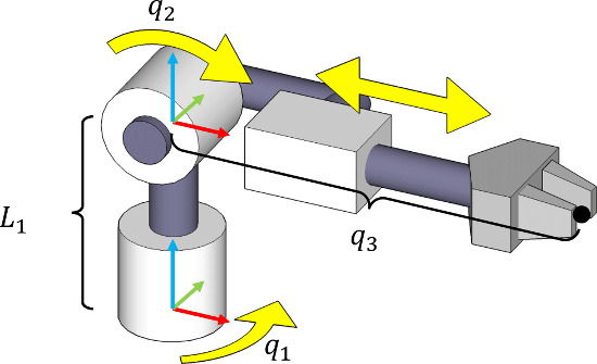
2RP manipulator
Consider a 2RP spherical manipulator whose first axis rotates about the $z$ axis, the second about the $y$ axis, and the prismatic joint translates about the $x$ axis. All reference frames are aligned with the world frame (that is, $L_1=0$ in Fig. 3).
With this definition, $T_{i,ref}^{p[i],ref} = I$ for each link. So, the transform of the third link is given by $$T_3(q) = \left[\begin{array}{ccc|c} & & & 0 \\ & R_z(q_1) & & 0 \\ & & & 0 \\ \hline 0 & 0 & 0 & 1 \end{array}\right] \left[\begin{array}{ccc|c} & & & 0 \\ & R_y(q_2) & & 0 \\ & & & 0 \\ \hline 0 & 0 & 0 & 1 \end{array}\right] \left[\begin{array}{ccc|c} & & & q_3 \\ & I & & 0 \\ & & & 0 \\ \hline 0 & 0 & 0 & 1 \end{array}\right]$$
The first two matrix multiplications compute the homogeneous representation of $$ R_z(q_1) R_y(q_2) = \left[\begin{array}{ccc} c_1 & -s_1 & 0 \\ s_1 & c_1 & 0 \\ 0 & 0 & 1 \end{array}\right] \left[\begin{array}{ccc} c_2 & 0 & s_2 \\ 0 & 1 & 0 \\ -s_2 & 0 & c_2 \end{array}\right] = \left[\begin{array}{ccc} c_1 c_2 & -s_1 & c_1 s_2 \\ s_1 c_2 & c_1 & s_1 s_2 \\ -s_2 & 0 & c_2 \end{array}\right]. $$
Hence, the final result is
$$T_3(q) = \left[\begin{array}{ccc|c} & & & \\ & R_z(q_1)R_y(q_2) & & R_z(q_1)R_y(q_2)\mathbf{e}_1 q_3 \\ & & & \\ \hline 0 & 0 & 0 & 1 \end{array}\right]$$where again we have used block matrix representation, and $\mathbf{e}_1 = (1,0,0)$. In other words, the origin of the third frame is: $$T_3(q)\left[\begin{array}{c}0 \\ 0 \\ 0 \\ 1\end{array}\right] = \left[\begin{array}{c} \\ R_z(q_1)R_y(q_2)\mathbf{e}_1 q_3 \\ \\ \hline 1 \end{array}\right] = \left[\begin{array}{c} c_1 c_2 q_3 \\ s_1 c_2 q_3 \\ -s_2 q_3 \\ 1 \end{array}\right].$$ Note that the vertical component of this point is proportional to the negative of $\sin q_2$, which may not be expected because $q_2$ could be mistakenly be considered to be an elevation angle of the translation axis. The reason is that rotations about the $y$ axis rotate CCW about the $(z,x)$ plane, not the $(x,z)$ plane. To change the interpretation so that $q_2$ measures the elevation angle, the second axis of rotation could be rotated so that $\mathbf{a}_2 = (0,-1,0)$, or equivalently, that the reference transform $T_{2,ref}$ rotates $\pi$ radians about either the $x$ or $z$ axis.
6R manipulator
Now consider a more typical 6R industrial robot arm, configured with the reference coordinate system as shown in Figure 4. (Ignore the gripper degree of freedom.) The shoulder axes and wrist axes intersect at a common point, indicated by the marked coordinate frames.

In this definition, the joint axes are aligned to the Z Y Y X Y Z axes, listed from the base to the end effector. All reference orientations are aligned to the world coordinate frame. The coordinate frames are also oriented such that positive joint angles turn counterclockwise with respect to their local coordinate frames, and hence we can more specifically list the joint axes as +Z +Y +Y +X +Y +Z.
Let us place the relative reference transforms so that both of the first 2 link transforms are at the intersection of the shoulder, and the last 3 link transforms are at the intersection of the wrist. All relative transforms have the identity matrix as their rotation component. Link 1's reference transform shifts by $L_1$ units in the Z direction, link 3 shifts by $L_2$ units in the X direction, and link 4 shifts by $L_3$ units the X direction, while links 2, 5, and 6 induce no translation.
Ultimately, forward kinematics yields the following transforms of each link:
$$T_1(q) = \left[\begin{array}{ccc|c} & & & 0 \\ & R_z(q_1) & & 0 \\ & & & L_1 \\ \hline 0 & 0 & 0 & 1 \end{array}\right] $$$$T_2(q) = T_1(q) \left[\begin{array}{ccc|c} & & & 0 \\ & R_y(q_2) & & 0 \\ & & & 0 \\ \hline 0 & 0 & 0 & 1 \end{array}\right] $$$$T_3(q) = T_2(q) \left[\begin{array}{ccc|c} & & & L_2 \\ & R_y(q_3) & & 0 \\ & & & 0 \\ \hline 0 & 0 & 0 & 1 \end{array}\right] $$$$T_4(q) = T_3(q) \left[\begin{array}{ccc|c} & & & L_3 \\ & R_x(q_4) & & 0 \\ & & & 0 \\ \hline 0 & 0 & 0 & 1 \end{array}\right] $$$$T_5(q) = T_4(q) \left[\begin{array}{ccc|c} & & & 0 \\ & R_y(q_5) & & 0 \\ & & & 0 \\ \hline 0 & 0 & 0 & 1 \end{array}\right] $$$$T_6(q) = T_5(q) \left[\begin{array}{ccc|c} & & & 0 \\ & R_z(q_6) & & 0 \\ & & & 0 \\ \hline 0 & 0 & 0 & 1 \end{array}\right] $$To obtain the world-space position of the end effector, we simply apply $T_6(q)$ to the local coordinates of the end effector in link 6's frame: $$\mathbf{x}(q) = T_6(q) \begin{bmatrix} L_6 \\ 0 \\ 0 \\ 1 \end{bmatrix}. $$
Kinematics conventions
As we defined the layout of a robot's kinematic structure above, we store the following parameters for each link $i=1,\ldots,n$: parents $p[i]$, reference relative transforms $T_{i,ref}^{p[i],ref}$, joint types $z_i$, and translational or rotational axes $\mathbf{a}_i$ .
However, our 2RP example showed that there are multiple choices of frames and axes that define the exact same robot dimensions. In fact, there are an infinite number of equivalent representations formed by modifying reference frames and joint axes so that the axes represent the same quantities in world coordinates. Moreover, we may rotate or translate a link's reference frame arbitrarily around its joint axis, as long as we correct for the shift in its zero position. For some purposes, it is useful to reduce the number of parameters specifying a robot's reference frame by choosing a convention. We have already seen a convention where we have chosen to place joint axes at the origin of the child frame; in general, the joint could have been placed arbitrarily in space.
Planar robot convention
We have also seen the standard convention for 2D planar robots in the $n$R example, in which we chose to align the reference frame with the $x$ axis. Here, by a change of world frame and zero positions, we need only represent the lengths between joints $L_0,L_1,...,L_n$. By a shift of the world frame, we could also eliminate the parameter $L_0$.
In the case where prismatic joints are present, we only need represent the direction of translation $\mathbf{a}_i$. But even these two parameters are excessive, since directions are unit vectors. Hence, we can simply represent the heading angle $\theta_i$ such that $\mathbf{a}_i = (\cos \theta_i, \sin \theta_i)$.
As a result, a minimum set of kinematic parameters for a 2D robot are the link lengths $L_1,\ldots,L_n$ and the headings of any translational axes $\theta_i$.
Denavit-Hartenberg convention
Denavit-Hartenberg convention is a well-known minimal parameter convention for 3D serial robot kinematics. In this convention, joint axes are always aligned to the $z$ axis of each child link, and the offset between joints is always pointing along the $x$ axis of the parent link. It is usually not the most convenient representation for the purposes of robot design and forward kinematics calculations, but due to the minimal number of parameters used (4 per link) it remains popular for robot structure optimization problems, like in robot calibration.
A single-pass forward kinematics algorithm
Forward kinematics can be computed through a single pass through the links, and for typical robots (at most hundreds of links), this process can be performed in a matter of microseconds.
To do so, we order links so that the parent occurs earlier in the ordering than $i$, i.e., $p[i] < i$. By convention, the base link is index 1 and has its parent equal to the world: $p[1] = W$. (Such an ordering exists, and can be calculated by a topological sort on the link graph, such as a depth first search.)
Forward kinematics can then be calculated as given as Algorithm 1:
Algorithm 1. Forward kinematics
$T_W(q) \gets I$.
For $i=1,\ldots,N$ in topologically sorted order:
Use ($\ref{eq:RecursiveForwardKinematicsGeneralized}$) to calculate $T_i(q)$ using the stored value of $T_{p[i]}(q)$.
Store $T_i(q)$.
Return $T_1,\ldots,T_N$
After the algorithm is complete, all link frames $T_1,\ldots,T_N$ are calculated with respect to the world frame.
Robot kinematic definition files
Although deriving a closed-form symbolic expression for forward kinematics is helpful for some purposes, it is often more convenient and less error-prone to let a software package calculate forward kinematics using Algorithm 1. These packages will use the kinematic parameters from a given robot specification (usually a file) for forward kinematics calculations.
ROS introduced the Universal Robot Description Format (URDF), which defines the kinematics of a robot (as well as masses, geometry, joint limits, and more) using an XML-based syntax. Although this was not the first type of robot file format, it became popularized due to the success of ROS, and now URDF files are widely used in many other robotics packages (including Klamp't). The main elements of URDF files are links and joints, given under the following structure:
<robot name="My 2R robot">
  <link name="base_link">
     ...
  </link>

  <link name="link_1">
     ...
  </link>

  <link name="link_2">
     ...
  </link>

  <joint name="joint_1" type="revolute">
    ...
    <parent link="base_link"/>
    <child link="link_1"/>
  </joint>

  <joint name="joint_2" type="revolute">
     ...
    <parent link="link_1"/>
    <child link="link_2"/>
  </joint>
</robot>
The ordering of links and joints in the file does not matter. Note that although this is only a 2R robot, there are actually three links including a privileged "base_link" that is attached to the world. Each joint connects two links, which are given by the "parent" and "child" attributes. URDF only supports robots with tree topology --- this is enforced by requiring a link to be a child of at most one joint. Somewhat contrary to our definition, there is no notion of a link's reference frame in URDF, and rather, reference frames are associated with 1) a link's inertial frame, 2) a link's visual geometry's frame, 3) link's collision geometry's frame, or 4) a joint. The closest analogue in URDF to our definition of a link's frame is actually the frame of the joint for which it is a child.
The link element contains three sub-elements: visual, collision, and inertial. Respectively, these describe the appearance of the link for visualization purposes, the shape of the link for collision detection purposes, and the link's inertial parameters, like it's mass and center of mass. An example of a grey cylinder extending 1 unit along the x axis is as follows:
<link name="link_1">
  <visual>
    <origin xyz="0 0 0" rpy="0 1.5708 0" />
    <geometry>
      <cylinder length="1" radius="0.1"/>
    </geometry>
    <material name="grey">
      <color rgba="0.6 0.6 .6 1"/>
    </material>
  </visual>
  <collision>
    <origin xyz="0 0 0" rpy="0 1.5708 0" />
    <geometry>
      <cylinder length="1.0" radius="0.1"/>
    </geometry>
  </collision>
  <inertial>
    <mass value="2.0"/>
    <inertia ixx="0.2" ixy="0.0" ixz="0.0" iyy="0.6" iyz="0.0" izz="0.6"/>
  </inertial>
</link>
Origins of frames are given in world coordinates, with roll-pitch-yaw convention for the orientation of each frame. We will discuss geometry and inertial properties in later chapters.
A joint can contain a number of items for simulation, but its primary sub-elements are as follows:
<joint name="joint_2" type="revolute">
  <origin xyz="1 0 0" rpy="0 0 0"/>
  <axis xyz="0 1 0"/>
  <parent link="link_1" />
  <child link="link_2" />
</joint>
The most relevant elements to the kinematic structure of a robot are the origin and axis elements, which respectively give the reference transform $T_{i}^{ref}$ and joint axis $\mathbf{a}_i$ (both in world coordinates).
Besides revolute and prismatic types, joints can also be of a "fixed" type, which simply attaches two links together, at the joint's frame of reference. This is often used in URDF files simply to define dummy frames that do not correspond to any moving part of the robot, but rather define useful reference frames attached to the robot, such as camera reference frames or end effector points. As an example, an end-effector frame for the 2R robot above could be defined with
<link name="end_effector">
</link>
<joint name="end_effector" type="fixed">
  <origin xyz="2 0 0"/>
</joint>
Several software libraries, such as Klamp't and Orocos KDL, will compute forward kinematics for any robot specified in URDF format. As an example in Klamp't, the following code prints the end effector position of the 2R robot given above at the configuration $(\pi/4,\pi/4)$:
#Code for doing basic forward kinematics with Klamp't
from __future__ import print_function,division
from klampt import *
import math
world = WorldModel()
res = world.readFile("data/planar2R.urdf")
assert res, "There was an error loading data/planar2R.urdf"
robot = world.robot(0)
#modifies the current configuration of the robot -- the 3rd element is just the end effector frame
robot.setConfig([math.pi/4,math.pi/4,0])
#returns the world coordinates of a point on link_2 whose local coordinates are [1,0,0]
print("World position of point at q=(pi/4,pi/4):",robot.link("link_2").getWorldPosition([1,0,0]))
#or, with the end effector frame added...
#getTransform() returns a pair (R,t) giving the rotation and translation of the
#end effector frame, so the R,t = ... syntax extracts the translation only
R,t = robot.link("end_effector").getTransform()
print("World position of the end_effector frame",t)
Note that Klamp't numbers the links as they are listed in the URDF file, and assigns a configuration degree-of-freedom to each link. Hence, the 4-element configuration provided in line 7 addresses the links base_link, link_1, link_2, and the dummy end_effector frame.
#This shows the robot and forward kinematics result↔
Summary
Key takeaways:
The kinematics of a robot relate the joint angles of a robot to the coordinate frames of its links.
A robot's configuration is a minimal expression of its links position, and usually consists of the robot's joint angles. The variables defining the configuration are the robot's degrees of freedom.
The topology of a robot structure is defined by its joint types (e.g., revolute, prismatic, and spherical) and how they are connected. Along with its link lengths and joint axes, this defines its kinematic structure.
A robot's reachable workspace is the range of end effector locations it could reach (and optionally orientations).
Forward kinematics computes the coordinate frames corresponding to robot's configuration. It can be computed for all links in a serial or branched robot with a single-pass algorithm.
Software for calculating forward kinematics should be available in any major robotics package.
Exercises
TODO...
Describe the configuration space of 1) a door (with a handle), 2) your arm, 3) a bicycle, 4) a car, and 5) your body while standing. How many links, joints, and closed loops do each system have? How many degrees of freedom are available in each system?
Suppose a 2R manipulator with unit link lengths and joint limits of $\pm 45^\circ$. Illustrate the workspace of its end effector position as precisely as possible. Then, illustrate the workspace of its end effector $y$ position and angle $\theta$.
Suppose in an $n$-link serial robot, we've computed all the frames for configuration $\mathbf{q}$. Now, suppose only one joint angle $i$ is changed from $q_i \rightarrow q_i^\prime$. What is the minimal number of operations that must we perform to determine $T_n(\mathbf{q}^\prime)$?
Implement a workspace approximation algorithm that takes a 6-link industrial robot as input, and calculates an approximate end-effector position workspace. You should loop through all combinations of joint angles within its joint range, up to a resolution of $10^\circ$, and for each configuration calculates the end effector position using forward kinematics. Output and plot these points using a 3D graphing program, such as Matlab or Excel. What kind of shape do the points approximate? How densely or sparsely is this shape sampled?
6DOF industrial manipulator